Ensemble Pruning for Glaucoma Detection in an Unbalanced Data Set
Werner Adler1, Olaf Gefeller1, Asma Gul2, Folkert K. Horn3, Zardad Khan4, Berthold Lausen5 1
Institute of Medical Informatics, Biometry, and Epidemiology, Friedrich-Alexander University Erlangen-Nuremberg, Erlangen, Germany
2
Department of Statistics, Shaheed Benazir Bhutto Women University, Peshawar, Pakistan 3
Department of Ophthalmology, Friedrich-Alexander University Erlangen-Nuremberg, Germany
4
Department of Statistics, Abdul Wali Khan University, Mardan, Pakistan 5
Department of Mathematical Sciences, University of Essex, Colchester CO4 3SQ, UK Corresponding Author:
Werner Adler ([email protected]), +49 9131 8525738, Waldstr. 6, 91054 Erlangen
This article is not an exact copy of the original published article in Methods of Information in Medicine. The definitive publisher-authenticated version of Adler, Werner and Gefeller, Olaf and Gul, Asma and Horn, Folbert K and Khan, Zardad and Lausen, Berthold (2016) 'Ensemble Pruning for Glaucoma Detection in an Unbalanced Data Set.' Methods of Information in Medicine, 55 (6). pp. 557-563. ISSN 0026-1270 is available online at:
Summary
Background: Random forests are successful classifier ensemble methods consisting of typically 100 to 1000 classification trees. Ensemble pruning techniques reduce the computational cost, especially the memory demand, of random forests by reducing the number of trees without relevant loss of performance or even with increased performance of the sub-ensemble. The application to the problem of an early detection of glaucoma, a severe eye disease with low prevalence, based on topographical measurements of the eye background faces specific challenges.
Objectives: We examine the performance of ensemble pruning strategies for glaucoma detection in an unbalanced data situation.
Methods: The data set consists of 102 topographical features of the eye background of 254 healthy controls and 55 glaucoma patients. We compare the area under the receiver operating characteristic curve (AUC), and the Brier score on the total data set, in the majority class, and in the minority class of pruned random forest ensembles obtained with strategies based on the prediction accuracy of greedily grown sub-ensembles, the uncertainty weighted accuracy, and the similarity between single trees. To validate the findings and to examine the influence of the prevalence of glaucoma in the data set, we additionally perform a simulation study with lower prevalences of glaucoma.
Results: In glaucoma classification all three pruning strategies lead to improved AUC and smaller Brier scores on the total data set with sub-ensembles as small as 30 to 80 trees compared to the classification results obtained with the full ensemble consisting of 1000 trees. In the simulation study, we were able to show that the prevalence of glaucoma is a critical factor and lower prevalence decreases the performance of our pruning strategies.
Conclusion: The memory demand for glaucoma classification in an unbalanced data situation based on random forests could effectively be reduced by the application of pruning strategies without loss of performance in a population with increased risk of glaucoma.
1. Introduction
Ensemble learning is a well-known strategy to deal with classification or regression problems [1, 2]. In the classification case, several classifiers are trained on the data and the ensemble decision, for example obtained by majority voting, often outperforms the best single classifier [3]. The success of ensemble strategies is based on the fact that the classification error of an ensemble can be explained by the average error of the single classifiers minus the diversity of the ensemble [4], i.e. a classification ensemble performs better when the single classifiers constituting the ensemble are not too similar to each other. One approach to create an ensemble is called bagging [5]. Here, several bootstrap samples are drawn from the learning data and a new classifier is trained on each sample. A random forest (RF) is a technique that utilizes bagging with classification trees [6]. An RF consists of classification trees where in each split node of the single trees only a random sample of all available variables is
considered to reduce the similarity between the trees. The trees constituting the ensemble are created considering different subsets of variables in their split nodes and thus are less
correlated, leading to a better performance of the total ensemble.
Typically, an RF consists of 100 to 1000 trees. Oshiro et al. [7] examined RF with a varying number of trees on 29 data sets and found that prediction accuracy was not significantly improved when they added more than 128 trees. Nevertheless, often several hundred or 1000 trees are used in an RF because increasing the number of trees in a random forest does not necessarily lead to overfitting of the data while too few trees tend to decrease the
classification performance. By default, trees in RF are fully grown, i.e. an RF tree consists of as many splits as are necessary to be able to classify each single observation in the training data set correctly. Thus, the memory demand of an RF can be high when a large number of trees is used and the training data set is large.
Ensemble pruning, i.e. the reduction of classifiers in ensembles, has been analysed
extensively in the literature [8-10]. The exact determination of the optimal sub-ensemble with the highest classification performance is computationally prohibitive for moderate ensemble sizes because of the high number of possible combinations. The selection of a near-optimal solution can be based on optimization techniques like genetic algorithms or semi-definite programming [11-14]. Stepwise forward selection, where a sub-ensemble is created by starting with a single-tree and adding one tree after the other, is a much faster way to search for well performing sub-ensembles, although the optimality of created sub-ensembles is not necessarily guaranteed and the global optimum almost certainly is not obtained. However, this strategy can lead to sub-ensembles performing well enough to justify this computationally less expensive approach. The selection of single classifiers can be based on the dissimilarity of the classifiers to each other to increase the diversity of the ensemble. The problem, how diversity in an ensemble or distances between classifiers can best be measured, is discussed extensively [15-19]. As the connection between several proposed diversity measures and the performance of the ensemble is not as straightforward as might be hoped [16, 19] and not always higher diversity leads to an improved ensemble [20], the classification performance of single classifiers also was considered for ensemble pruning [21-23]. Another criterion
discussed for ensemble pruning is the classification margin [24].
In this work, we apply ensemble pruning techniques to a two-class classification problem in medical research [25-27], the identification of glaucomatous observations based on
topographical measurements of the eye background. Because of the low prevalence of glaucoma on the population level, unbalanced data sets are an issue in glaucoma screening programs. We call a data set unbalanced, if the distribution over the two classes deviates strongly from a uniform distribution. Unmodified application of classification techniques that
are trained to minimize the classification error in this case will lead to classifiers with a high specificity and low sensitivity, as the classification error is dominated by the misclassification of the majority class (the class with more observations, i.e. normal) and less affected by misclassifications in the minority class (the class with fewer observations, i.e. glaucoma). We deal with this situation by applying the SMOTE strategy [28] and setting the class weight parameter of the RF. The class membership probability predicted by the random forests is evaluated rather than the class.The prediction performances in both classes thus can be
reported with class-specific Brier scores[29]. In our clinical glaucoma data set, the prevalence of glaucoma is 18%, which is substantially higher than on the population level. To examine the influence of the prevalence on the performance of the pruning strategies, we additionally perform a simulation study with lower prevalences.
The remaining paper is organized as follows: in subsection 2.1 we describe the pruning strategies, and in subsections 2.3 and 2.4 we introduce the glaucoma data set and give a description of our simulation study, respectively. The results are presented in section 3 and a discussion is given in section 4.
2. Methods
The pruning strategies and experiments described in this section were implemented using the statistical programming language R [30]. We used the implementation given in the package randomForest to build RF style classification trees. The tree predictions were stored in a list structure for further processing by pruning strategies implemented following the respective descriptions in the literature (see Online Appendix A – RF Framework for an overview). 2.1. Ensemble Pruning
In a first step, we train a standard random forest consisting of 1000 trees. To diminish the problem of an unbalanced data set the synthetic minority over-sampling technique (SMOTE) proposed by Chawla et al. [28] is applied and the a priori probabilities of the classes are specified by the RF class weight parameter (see Online Appendix B – Unbalanced Data). Then, we aim to reduce the number of trees in the RF. Not only does this reduce the memory demand of the classifier (see Online Appendix C – Computational Cost) but a more
parsimonious ensemble may also lead to an improved performance.
Tsoumakis et al. have identified conceptually different main strategies of ensemble pruning [10]. One approach is to tackle the pruning problem by optimization-based methods. These computationally expensive methods formulate the problem of identifying a near-optimal sub-ensemble as optimization problem. Commonly known approaches are genetic algorithms or semi-definite programming [11, 12]. A different way to reduce the number of trees is covered by clustering-based methods. Here, similar trees are identified using clustering-techniques and the trees constituting the final sub-ensemble are chosen from these clusters [31].
Our focus lies on a third strategy, the greedy stepwise growth of ensembles based on the evaluation of sub-ensembles or single trees. One characteristic of this approach is that the size of the new ensemble is not automatically determined but the performances of all sub-ensembles of an increasing number of trees can be evaluated. The size of the ensemble finally used can be specified either taking memory restrictions into account or focusing on the
performance of the sub-ensemble. In the next subsections we provide a detailed description of those pruning strategies considered further in our evaluation. Our selection of pruning
methods is by no means comprehensive. Several modifications and variants of these strategies as well as related pruning methods have been considered in previous work [9, 11, 12, 24, 32, 33].
2.1.1 Pruning by Prediction Accuracy: Brier Score
The Brier score is a measure that can be used to calculate the quality of probabilistic predictions as those obtained by RFs, where the fraction of trees voting for a specific class membership can be interpreted as a probability. Assuming we estimate the probability for a truly non-glaucomatous observation to belong to the class “glaucoma”, the optimal
probability 𝑜𝑜𝑖𝑖 of this observation 𝑖𝑖 is zero; conversely, for a glaucomatous observation the optimal probability is 1. The Brier score then is simply calculated as the mean squared difference between the predicted probabilities and the optimal probabilities over all observations.
As each single tree in an RF is trained only on a subset of the training data, for each tree there are so-called out-of-bag observations, i.e. observations that were not used in the training process and that can be used to estimate the predictive performance of the tree “for free”, i.e. without having to rely on additional test data not in the training set. This allows for the out-of-bag estimation of the Brier score 𝐵𝐵𝐵𝐵�𝑜𝑜𝑜𝑜𝑜𝑜:
𝐵𝐵𝐵𝐵�𝑜𝑜𝑜𝑜𝑜𝑜 =𝑁𝑁 �1 (𝑝𝑝𝑜𝑜𝑜𝑜𝑜𝑜,𝑖𝑖 − 𝑜𝑜𝑖𝑖) 𝑖𝑖
2
, 𝑖𝑖= 1, … ,𝑁𝑁
Here 𝑝𝑝𝑜𝑜𝑜𝑜𝑜𝑜,𝑖𝑖 is the out-of-bag probability for observation 𝑖𝑖, i.e.the fraction of the trees voting for the class “glaucoma” among all trees generated without observation 𝑖𝑖. 𝑁𝑁 denotes the size of the learning set.
Pruning based on the Brier score is performed in the following way: first, the tree with lowest out-of-bag error is selected as “seed” for the ensemble. The out-of-bag error of a tree is the fraction of false predictions among observations in the out-of-bag set of the respective tree. Then, Brier scores for all sub-ensembles of size two consisting of this “seed” and one of the remaining trees of the original ensemble are calculated. That sub-ensemble leading to the smallest Brier score replaces the “seed” and the process of growing the sub-ensemble is iterated until a fixed size is reached or until all trees are in the ensemble.
In the course of our work, we not only examined pruning based on the Brier score with the total data set but also analysed pruning based on the Brier score in the minority class to improve the accuracy in the minority class. However, although the Brier score in the minority class was substantially improved, the performance on the total data set as measured by AUC and Brier score was worsened dramatically. Therefore, we skipped the results following this strategy.
2.1.2 Pruning by Uncertainty Weighted Accuracy: UWA
Partalas et al.[23] introduced a promising measure to direct ensemble pruning. In addition to the prediction performance of a classification tree, this measure is based on the prediction uncertainty of the hitherto existing sub-ensemble when evaluating trees that should be added to the sub-ensemble. This uncertainty simply is estimated by the non-uniformity of decisions of trees constituting the (sub-)ensemble. Therefore, we define 𝑁𝑁𝑁𝑁𝑖𝑖 as the proportion of trees in ensemble 𝐸𝐸 that classify observation 𝑖𝑖 correctly and 𝑁𝑁𝑁𝑁𝑖𝑖 as the proportion of trees that
classify this observation incorrectly. The trees in question to be added to the sub-ensemble then are weighted in following way: Trees gain positive weight or a reward for each
classify incorrectly. The height of the reward (or the penalty) for an observation is determined by the uncertainty of the ensemble 𝐸𝐸 classifying this observation: if 𝐸𝐸 classifies the
observation correctly, the reward (or penalty) is given by (−)𝑁𝑁𝑁𝑁𝑖𝑖 and if 𝐸𝐸classifies the observation incorrectly, the reward (or penalty) is determined by (−)𝑁𝑁𝑁𝑁𝑖𝑖. The uncertainty weighted accuracy UWA of the tree is the average reward/penalty over all observations. For an out-of-bag estimation of the UWA, 𝑁𝑁𝑁𝑁𝑖𝑖 and 𝑁𝑁𝑁𝑁𝑖𝑖 are replaced by the respective fractions of trees producing out-of-bag predictions for observation 𝑖𝑖 and the UWA is averaged over those observations, for which the tree and the ensemble produce out-of-bag predictions.
2.1.3 Pruning by diversity: the Double-Fault measure (DF)
The Double-Fault (DF) similarity can be calculated to measure the similarity between two classifiers [16]. It can be understood as a pairwise similarity between two trees based on their predictions of observations. The trees are defined to be more similar, if they both more frequently misclassify the same observations. To be able to calculate the DF measure, one needs to know the true classes of the observations. The comparison of the predicted classes with the true classes can be done using so-called oracle predictions [16]. An oracle prediction is defined to be 1, if the predicted class is true and 0, if the predicted class is false. Comparing two classification trees 𝑡𝑡1 and 𝑡𝑡2, we can define 𝑛𝑛𝑖𝑖,𝑗𝑗 as the number of observations, for which the oracle predictions of 𝑡𝑡1 are 𝑖𝑖 and of 𝑡𝑡2 are 𝑗𝑗, respectively (𝑖𝑖,𝑗𝑗 ∈{0,1}). In particular, 𝑛𝑛0,0 can be defined as the number of observations, for which both trees predict the false class. The estimated DF similarity 𝐷𝐷𝑁𝑁�(𝑡𝑡1,𝑡𝑡2) between two trees 𝑡𝑡1 and 𝑡𝑡2 then is:
𝐷𝐷𝑁𝑁�(𝑡𝑡1,𝑡𝑡2) = 𝑛𝑛 0,0
𝑛𝑛0,0+𝑛𝑛0,1+𝑛𝑛1,0+𝑛𝑛1,1
This is the fraction of the number of false predictions of two trees among the total number of predictions. The DF similarity is defined only for two classifiers, the mean DF similarity 𝐵𝐵𝑆𝑆𝑆𝑆� 𝐷𝐷𝐷𝐷(𝑡𝑡𝑖𝑖) of any tree 𝑡𝑡𝑖𝑖 to all other 𝑛𝑛𝑡𝑡𝑛𝑛𝑛𝑛𝑛𝑛 −1 trees can be calculates as:
𝐵𝐵𝑆𝑆𝑆𝑆� 𝐷𝐷𝐷𝐷(𝑡𝑡𝑖𝑖) =𝑛𝑛𝑡𝑡𝑛𝑛𝑛𝑛𝑛𝑛 −1 1 � 𝐷𝐷𝑁𝑁� �𝑡𝑡𝑖𝑖,𝑡𝑡𝑗𝑗� 𝑗𝑗≠𝑖𝑖
Because a diverse RF ensemble consists of trees that are as distant to the other trees as possible, this mean similarity 𝐵𝐵𝑆𝑆𝑆𝑆� 𝐷𝐷𝐷𝐷(𝑡𝑡𝑖𝑖) then may be used as a measure to assess the quality of a single tree (the smaller the similarity, the better the tree). We are aware that simple aggregation of trees based on this measure does not necessarily lead to the selection of the n
most distant trees when we choose the n trees with smallest 𝐵𝐵𝑆𝑆𝑆𝑆� 𝐷𝐷𝐷𝐷(𝑡𝑡𝑖𝑖) but we point out the attractiveness of this approach because of its simplicity. As with the Brier score, we use the out-of-bag data to assess the DF similarity between all classification trees. Thus, we do not need additional tuning data. The similarity between two trees then is determined by the intersection of the out-of-bag observations of both trees and instead of using all observations 𝑛𝑛𝑖𝑖,𝑗𝑗 only observations in this intersection set are used, denoted as 𝑛𝑛
𝑜𝑜𝑜𝑜𝑜𝑜(𝑡𝑡1,𝑡𝑡2)𝑖𝑖,𝑗𝑗:
𝐷𝐷𝑁𝑁�𝑜𝑜𝑜𝑜𝑜𝑜(𝑡𝑡1,𝑡𝑡2) = 𝑛𝑛𝑜𝑜𝑜𝑜𝑜𝑜(𝑡𝑡1,𝑡𝑡2)
0,0
𝑛𝑛𝑜𝑜𝑜𝑜𝑜𝑜(𝑡𝑡1,𝑡𝑡2)0,0+𝑛𝑛𝑜𝑜𝑜𝑜𝑜𝑜(𝑡𝑡1,𝑡𝑡2)0,1+𝑛𝑛𝑜𝑜𝑜𝑜𝑜𝑜(𝑡𝑡1,𝑡𝑡2)1,0+𝑛𝑛𝑜𝑜𝑜𝑜𝑜𝑜(𝑡𝑡1,𝑡𝑡2)1,1
2.1.4 Random Selection
To be able to assess the performance gain of the pruning strategies we created a random ordering of all trees and then use it to construct random reference sub-ensembles.
2.2 Clinical Data Set: Glaucoma Classification with HRT measurements
The data set consists of 254 observations of healthy controls and of 55 observations from patients with open-angle glaucoma. The set of variables comprises 102 features from the Heidelberg Retina Tomograph which produces three dimensional laser scanning images of the eye background and then calculates topographical features of these images. The data set is a combination of two case-control studies performed at the Erlangen University Eye Hospital described in more detail in Horn et al. [26] to examine the predictive power for glaucoma detection. In contrast to Horn et al. we used only those glaucomatous observations that were part of the test data in [26]. Thus, the glaucoma prevalence in our data set was reduced, motivated by the low prevalence of glaucoma which is a problem in population based glaucoma screening [34]. We calculated the area under the receiver operating characteristic curve (AUC) and the Brier score as measures of the overall classification performance. Due to the imbalanced classes, we also investigated the Brier score in the majority class and in the minority class, respectively, to analyse the class-specific performances. The performances were estimated by a ten times repeated ten-fold cross-validation.
2.3 Simulation Experiment
The influence of a reduced prevalence of glaucoma in the data set was examined further in a simulation experiment. The simulation study is based on the glaucoma data set described in the previous section. We assumed a multivariate normal distribution of the HRT variables with different location and scale parameters in the normal and glaucoma class. These
parameters were estimated from the clinical data set by the class-specific means and standard deviations, respectively. New observations are simulated by drawing randomly from these distributions. Such a simulation experiment allows for the extensive examination of the influence of unbalanced classes in data sets with lower prevalences.
Our simulation study consists of three settings where always a total of 200 observations is generated, but the number of observations belonging to the glaucoma class is varied from 30 (=15%, setting A) to 20 (=10%, setting B) to 10 (=5%, setting C). Each simulation setting consists of 100 simulation runs, where in each run one training set and one equally structured test set are simulated.
3. Results
The comparison between pruning strategies and a full RF consisting of 1000 trees should not only focus on performance differences, but also assess differences in computational costs, i.e. memory demand and runtime. When performance measures of a full RF and of some pruning methods are similar, the latter criteria play an important role when deciding whether RFs should be pruned or not. In our case, however, a comprehensive evaluation of differences in computational costs is currently not possible due to the lack of a computationally efficient implementation allowing a fair comparison of pruned RFs with full RFs. As a first step, we performed a conceptual comparison of different RFs of varying sizes to address the
computational aspect (see Online Appendix C – Computational Cost). The results reported in this section, however, refer only to the performances of the pruning strategies.
3.1 Glaucoma Classification
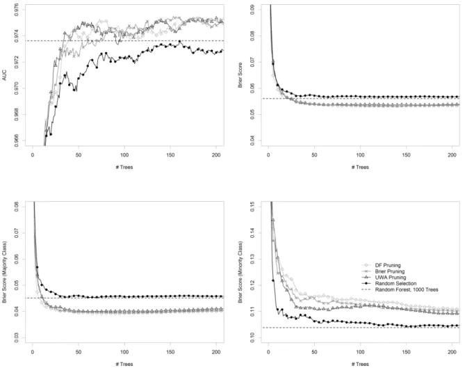
Figure 1 shows the AUC, and the Brier score with the total data set and in both classes separately of ensembles consisting of up to 200 trees built following the strategies described in the previous section. Three of four measures (AUC, Brier Score, Brier Score (Majority Class)) can very clearly be improved with our pruning strategies. With DF and UWA pruning,
the AUC of the full RF consisting of 1000 trees is already achieved with ensembles consisting of about 50 trees, and with Brier pruning, ensembles with about 80 trees yield a comparable AUC. The Brier scores are very similar for all three pruning strategies. On the total data set the Brier score of the full RF is obtained with about 30 trees, while the Brier score in the majority class already can be improved with an ensemble size larger than 20 trees. Moreover, the AUC plot and the Brier Score estimated from the total data set show that the
improvement obtained by our pruning strategies in the majority class overcompensates the weaker Brier score in the minority class compared to the full RF.
Figure 1: Classification results obtained with the glaucoma data set: AUC, Brier score on the total data set (top row, from left to right), Brier score in the majority class, and Brier score in the minority class (bottom row, from left to right) for ensembles consisting of 1 to 200 trees where the trees are selected based on the three examined strategies DF pruning, Brier pruning, and UWA pruning and performing random selection.
3.2 Simulation Experiment
A detailed report of the results in the simulation experiments, together with tables showing the AUC, and Brier scores for the total data set, for the majority class, and for the minority class
for random forests of sizes 50, 75, 100, 150, and 200 trees produced by pruning and the full RF consisting of 1000 trees are given in Online Appendix D – Simulation Results.
Overall, the performance of all three pruning strategies is very similar and a performance deterioration of these strategies can be observed as the prevalence is reduced.
In simulation setting A with a prevalence of 15%, all three pruning strategies are able to achieve the AUC, and the Brier score obtained with the full RF consisting of 1000 trees already with ensembles of size 50 and are even able to improve the overall performance and the performance in the majority class with ensembles sizes larger than 75 trees. A ranking in the performances of the different pruning strategies shows that – although results are very similar and absolute differences are negligible - in 15 cases (three measures: AUC, Brier score, Brier score in the majority class; five ensemble sizes) DF pruning produces best results, followed by Brier pruning, and finally by UWA pruning. The fact that none of the pruning strategies can improve random selection in the minority class highlights the importance of the performance in the majority class, even though the unbalanced data set was considered in training by applying SMOTE and by weighting the classes in the RF.
In setting B, the AUC of the full RF cannot be obtained with pruning strategies and an ensemble size of 50 trees. From 75 trees on, however, this AUC (0.982) is reached by DF pruning and by Brier pruning. UWA pruning still is a bit worse. With larger ensembles from 100 trees on, all three pruning strategies obtain the AUC of the full RF and even are able to improve it slightly. The Brier score estimated from the total data set and that in the majority class obtained by the full RF is improved with all three pruning strategies and all ensemble sizes by up to 26% (from 0.027 to 0.020), surprisingly even more pronounced in the smaller ensembles. The Brier score in the minority class of the full RF, however, is lower than that of all pruning strategies: 0.11 (full RF) compared to 0.127, 0.131, 0.133 (50 trees, UWA
pruning, Brier pruning, DF pruning, respectively), or 0.123 (all three strategies, 200 trees). In setting C with 5% prevalence, all three pruning strategies can improve the overall Brier score and the Brier score in the majority class compared to the full RF. As in setting A and B, however, the Brier score in the minority class obtained with the full RF is lower than that obtained by all three pruning strategies. The AUC of the full RF is obtained by DF pruning from 75 trees on and from UWA pruning and Brier pruning from 150 trees on.
4. Discussion
Random forests have already demonstrated their ability to yield good results for glaucoma classification based on topography information of the eye background [25, 26]. In this work, we were interested in the reduction of the computational cost of these classifiers by the
application of pruning strategies. The performance of pruned RFs in unbalanced data sets with a low glaucoma prevalence was of special interest because of the need to improve classifier performance for population-based glaucoma screening programs [35].
One pruning strategy evaluated in our work is based on the similarity of trees to increase the ensemble diversity, as this is known to play a major part in the success of ensemble learning [4, 20]. The similarity of classifiers can be measured in many ways [16, 19]. However, we found very promising results using the DF similarity. It has been shown that classification performance of individual classifiers can play an important role in ensemble pruning [21, 22]. Partalas et al. [23] examined a more refined measure that is not only based on the tree
accuracy but also weighted with the ensemble uncertainty. This measure, UWA, showed also very competitive results in our glaucoma data set as well as in the simulation study. Our third measure is based on the accuracy of the probabilistic prediction, as measured by the Brier score. Although in some way simpler than DF or UWA, as no two predictions have to be
compared, but only the probabilistic outcome and the optimal probability, the Brier score also leads to very good pruning results.
In the simulation study, the performance of these pruning strategies was better at higher prevalences (10% and 15%). In setting C with a low prevalence of 5%, pruning reduces the computational cost, i.e. the memory demand, but cannot improve the performance of the full ensemble. On the other hand, the classification performance is still not jeopardised by pruning in this setting. However, a higher benefit of the application of pruning strategies can be
expected when applied to glaucoma data from high risk populations where the prevalence of glaucoma is higher than in setting C. Then, the classification performance of a fully grown RF consisting of 1000 trees can even be improved.
Although the complexity in the final ensembles once they are pruned is reduced, the higher effort that is necessary for training the ensembles has to be taken into account. In real world applications, however, training a classifier in most cases is a one time job and the trained classifier is then applied very often and has to prove its usefulness. Thus, reduced complexity in the classification step outweighs higher complexity in the training step by far. Therefore, our work can be seen as a preliminary examination of the feasibility of pruning strategies for RF. For practical applications, however, an efficient implementation of pruning strategies to RF is required, e.g. by providing an interface to an existing RF implementation.
A very interesting approach to reduce the computational cost in the classification step is given by Schwing et al. [36]. Based on statistical reasoning, they suggest an early termination of the classification process, when the class membership is reasonably sure.
Krawczyk et al.[37] also incorporated the DF measure to direct the pruning strategy in unbalanced data. In later work [38], they proposed an evolutionary algorithm based approach and achieved good performance. Bhowan et al. [11] implemented genetic programming to obtain optimal sub-ensembles with unbalanced data. It might be interesting to examine the difference between the pruning approaches considered here and these more complex optimization based proposals.
Acknowledgements:
We acknowledge support from grant number ES/L011859/1, from The Business and Local Government Data Research Centre, funded by the Economic and Social Research Council to provide researchers and analysts with secure data services.
References
1. Dietterich TG. Ensemble methods in machine learning. Multiple classifier systems: Springer; 2000.
2. Mayr A, Binder H, Gefeller O, Schmid M. The evolution of boosting algorithms. From machine learning to statistical modelling. Meth Inform Med. 2014;53(6):419-27.
3. Opitz D, Maclin R. Popular ensemble methods; An empirical study. Journal of Artificial Intelligence Research. 1999;11:169-98.
4. Krogh A, Vedelsby J. Neural network ensembles, cross validation, and active learning. Advances in Neural Information Processing Systems. Cambridge: MIT Press; 1995.
5. Breiman L. Bagging predictors. Machine Learning. 1996;24(2):123-40. 6. Breiman L. Random Forests. Machine Learning. 2001;45(1):5-32.
7. Oshiro T, Perez P, Baranauskas J. How many trees in a random forest? Machine Learning and Data Mining in Pattern Recognition. 2012:154-68.
9. Kulkarni VY, Sinha PK. Pruning of random forest classifiers: a survey and future directions. Data Science & Engineering (ICDSE), 2012 International Conference on. 2012:64-8.
10. Tsoumakas G, Partalas I, Vlahavas I. An ensemble pruning primer. Applications of supervised and unsupervised ensemble methods: Springer; 2009. p. 1-13.
11. Bhowan U, Johnston M, Zhang M. Ensemble learning and pruning in multi-objective genetic programming for classification with unbalanced data. AI 2011: Advances in Artificial Intelligence: Springer; 2011. p. 192-202.
12. Zhang Y, Burer S, Street WN. Ensemble pruning via semi-definite programming. The Journal of Machine Learning Research. 2006;7:1315-38.
13. Zhang L, Zhou WD. Sparse ensembles using weighted combination methods based on linear programming. Pattern Recognition. 2011;44(1):97-106.
14. Zhang J, Chau KW. Multilayer Ensemble Pruning via Novel Multi-sub-swarm Particle Swarm Optimization. J UCS. 2009;15(4):840-58.
15. Gatnar E. A diversity measure for tree-based classifier ensembles. Data Analysis and Decision Support: Studies in Classification, Data Analysis, and Knowledge Organization. 2005:30-8.
16. Kuncheva LI, Whitaker CJ. Measures of diversity in classifier ensembles and their relationship with the ensemble accuracy. Machine Learning. 2003;51(2):181-207.
17. Miglio R, Soffritti G. The comparison between classification trees through proximity measures. Computational Statistics & Data Analysis. 2004;45(3):577-93.
18. Norsida H, Bakri M, Norwati M, Rizam ABM. Similarity measure exercise for classification trees based on the classification path. Applied Mathematics and Computational Intelligence. 2012;1:33-41.
19. Tang EK, Suganthan PN, Yao X. An analysis of diversity measures. Machine Learning. 2006;65(1):247-71.
20. Brown G, Kuncheva LI. ''Good'' and ''bad'' diversity in majority vote ensembles. Multiple classifier systems: Springer; 2010. p. 124-33.
21. Gul A, Perperoglou A, Khan Z, Mahmoud O, Miftahuddin M, Adler W, et al. Ensemble of a subset of kNN classifiers. Advances in Data Analysis and Classification. 2016:1-14.
22. Khan Z, Gul A, Perperoglou A, Miftahuddin M, Mahmoud O, Adler W, et al. An ensemble of optimal trees for class membership probability estimation. Analysis of Large and Complex Data, European Conference on Data Analysis, July, 2014; Bremen: Springer; in press.
23. Partalas I, Tsoumakas G, Vlahavas I. An ensemble uncertainty aware measure for directed hill climbing ensemble pruning. Machine Learning. 2010;81:257-82.
24. Yang F, Lu W, Luo L, Li T. Margin optimization based pruning for random forest. Neurocomputing. 2012;94:54-63.
25. Adler W, Peters A, Lausen B. Comparison of classifiers applied to confocal scanning laser ophthalmoscopy data. Meth Inform Med. 2008;47:38-46.
26. Horn FK, Lämmer R, Mardin CY, Jünemann AG, Michelson G, Lausen B, et al. Combined evaluation of frequency doubling technology perimetry and scanning laser ophthalmoscopy for glaucoma detection using automated classification. Journal of Glaucoma. 2012;21(1):27-34. 27. Bowd C, Hao J, Tavares IM, Medeiros FA, Zangwill LM, Lee TW, et al. Bayesian machine learning classifiers for combining structural and functional measurements to classify healthy and glaucomatous eyes. Investigative Ophthalmology & Visual Science. 2008;49(3):945-53.
28. Chawla NV, Bowyer KW, Hall LO, Kegelmeyer WP. SMOTE: Synthetic Minority Over-Sampling Technique. Journal of Artificial Intelligence Research. 2002;16:321-57.
29. Wallace BC, Dahabreh IJ. Improving class probability estimates for imbalanced data. Knowledge and Information Systems. 2014;41(1):33-52.
30. R Core Team. R: A language and environment for statistical computing. R Foundation for Statistical Computing. 2015. Vienna, Austria.
31. Giacinto G, Roli F, Fumera G. Design of effective multiple classifier systems by clustering of classifiers. 15th International Conference on Pattern Recognition, ICPR 2000:160-3.
32. Lu Z, Wu X, Zhu X, Bongard J. Ensemble Pruning via Individual Contribution Ordering. Proceedings of the 16th ACM SIgKDD international conference on Knowledge discovery and data mining. 2010.
33. Martinez-Munoz G, Hernandez-Lobato D, Suarez A. An Analysis of Ensemble Pruning Techniques Based on Ordered Aggregation. TPAMI. 2009;31(2):245-59.
34. Tham Y, Li X, Wong T, Quigley H, Aung T, Cheng C. Global Prevalence of Glaucoma and Projections of Glaucoma Burden through 2040. Ophthalmology. 2014;121(11):2081-90.
35. Todd A, Müller A, Rait J, Keeffe J, Taylor H, Mukesh B. Performance of Community-Based Glaucoma Screening Using Frequency Doubling Technology and Heidelberg Retinal Tomography. Ophthalmic Epidemiology. 2005;12(3):167-78.
36. Schwing AG, Zach C, Zheng Y, Pollefeys M. Adaptive random forest - How many ''experts'' to ask before making a decision? Computer Vision and Pattern Recognition (CVPR), 2011 IEEE
Conference on. 2011:1377-84.
37. Krawczyk B, Schaefer G. An improved ensemble approach for imbalanced classification problems. Applied Computational Intelligence and Informatica (SACI), 2013 IEEE 8th International Symposium on. 2013:423-6.
38. Krawczyk B, Wozniak M, Schaefer G. Cost-sensitive decision tree ensembles for effective imbalanced classification. Applied Soft Computing. 2014;14:554-62.