www.kuleuven.be
KU LEUVEN
Inverse eigenvalue problems for extended Hessenberg
and extended tridiagonal matrices
Thomas Mach, Raf Vandebril, and Marc Van Barel
Thomas Mach
Department of Computer
Science
KU Leuven, Belgium
[email protected]
Raf Vandebril
Department of Computer
Science
KU Leuven, Belgium
[email protected]
Marc Van Barel
Department of Computer
Science
KU Leuven, Belgium
[email protected]
Abstract
In inverse eigenvalue problems one tries to reconstruct a matrix, satis-fying some constraints, given some spectral information. Here, two inverse eigenvalue problems are solved.
First, given the eigenvalues and the first components of the associated eigenvectors (called the weight vector) an extended Hessenberg matrix with prescribed poles is computed possessing these eigenvalues and satisfying the eigenvector constraints. The extended Hessenberg matrix is retrieved by ex-ecuting particularly designed unitary similarity transformations on the diag-onal matrix containing the eigenvalues. This inverse problem closely links to orthogonal rational functions: the extended Hessenberg matrix contains the recurrence coefficients given the nodes (eigenvalues), poles (poles of the extended Hessenberg matrix), and a weight vector (first eigenvector compo-nents) determining the discrete inner product. Moreover, it is also sort of the inverse of the (rational) Arnoldi algorithm: instead of using the (rational) Arnoldi method to compute a Krylov basis to approximate the spectrum, we will reconstruct the orthogonal Krylov basis given the spectral info.
In the second inverse eigenvalue problem, we do the same, but refrain from unitarity. As a result we execute possibly non-unitary similarity transforma-tions on the diagonal matrix of eigenvalues to retrieve a (non)-symmetric
extended tridiagonalmatrix. The algorithm will be less stable, but it will be faster, as the extended tridiagonal matrix admits a low cost factorization of
O(n) (nequals the number of eigenvalues), whereas the extended Hessenberg matrix does not. Again there is a close link with orthogonal function the-ory, the extended tridiagonal matrix captures the recurrence coefficients of bi-orthogonal rational functions. Moreover, it is again sort of inverse of the nonsymmetric Lanczos algorithm: given spectral properties, we reconstruct the two basis Krylov matrices linked to the nonsymmetric Lanczos algorithm
Article information
• Mach, Thomas; Vandebril, Raf; Van Barel, Marc. Inverse eigenvalue problems for extended Hessenberg and extended tridiagonal matrices, Journal of Computational and Applied Mathematics, volume 272, pages 377-398, 2014.
• The content of this article is identical to the content of the published paper, but without the final typesetting by the publisher.
• Journal’s homepage:
http://www.journals.elsevier.com/journal-of-computational-and-applied-mathematics/ • Published version: http://dx.doi.org/10.1016/j.cam.2014.03.015
HESSENBERG AND EXTENDED TRIDIAGONAL MATRICES
THOMAS MACH†, MARC VAN BAREL†, AND RAF VANDEBRIL†
Abstract. In inverse eigenvalue problems one tries to reconstruct a matrix, satisfying some
constraints, given some spectral information. Here, two inverse eigenvalue problems are solved. First, given the eigenvalues and the first components of the associated eigenvectors (called the weight vector) an extended Hessenberg matrix with prescribed poles is computed possessing these eigenvalues and satisfying the eigenvector constraints. The extended Hessenberg matrix is retrieved by executing particularly designed unitary similarity transformations on the diagonal matrix con-taining the eigenvalues. This inverse problem closely links to orthogonal rational functions: the extended Hessenberg matrix contains the recurrence coefficients given the nodes (eigenvalues), poles (poles of the extended Hessenberg matrix), and a weight vector (first eigenvector components) de-termining the discrete inner product. Moreover, it is also sort of the inverse of the (rational) Arnoldi algorithm: instead of using the (rational) Arnoldi method to compute a Krylov basis to approximate the spectrum, we will reconstruct the orthogonal Krylov basis given the spectral info.
In the second inverse eigenvalue problem, we do the same, but refrain from unitarity. As a result we execute possibly non-unitary similarity transformations on the diagonal matrix of eigenvalues to retrieve a (non)-symmetricextended tridiagonalmatrix. The algorithm will be less stable, but it will be faster, as the extended tridiagonal matrix admits a low cost factorization ofO(n) (nequals the number of eigenvalues), whereas the extended Hessenberg matrix does not. Again there is a close link with orthogonal function theory, the extended tridiagonal matrix captures the recurrence coefficients of bi-orthogonal rational functions. Moreover, it is again sort of inverse of the nonsymmetric Lanczos algorithm: given spectral properties, we reconstruct the two basis Krylov matrices linked to the nonsymmetric Lanczos algorithm
Key words.rational nonsymmetric Lanczos, rational Arnoldi, inverse eigenvalue problem, data
sparse factorizations, extended Hessenberg matrix
AMS subject classifications. 65F18, 65F25, 65F60, 65D32
1. Introduction. In this manuscript special instances of the following very gen-eral inverse eigenvalue problem are solved.
Definition 1.1 (Inverse Eigenvalue Problem, IEP-general). Given n complex
numbers λi and corresponding positive real weights wi, i= 1,2, . . . , n. Without loss
of generality, we will assume that the vector w= [w1, w2, . . . , wn] has 2-norm equal
to1. Find a matrixM having a certain desired structure such that the eigenvalues of
M are λi and such that the first component of the corresponding unit eigenvector is
wi.
This inverse eigenvalue problem computes the recurrence coefficients of orthog-onal functions, orthogorthog-onal with respect to a discrete inner product with the λi as
nodes and the |wi|2 as weights of the inner product. Solving such inverse
eigen-value problems, i.e. computing the recurrences and orthogonal functions (stemming from polynomials, Laurent polynomials, rational functions with finite and/or infinite
∗This research was supported in part by the Research Council KU Leuven, projects OT/11/055
(Spectral Properties of Perturbed Normal Matrices and their Applications), OT/10/038 (Multi-Parameter Model Order Reduction and its Applications), CoE EF/05/006 Optimization in En-gineering (OPTEC); by the Fund for Scientific Research–Flanders (Belgium) project G034212N (Reestablishing Smoothness for Matrix Manifold Optimization via Resolution of Singularities), by the Interuniversity Attraction Poles Programme, initiated by the Belgian State, Science Policy Office, Belgian Network DYSCO (Dynamical Systems, Control, and Optimization); and by a DFG research stipend MA 5852/1-1.
†Department of Computer Science, KU Leuven, 3001 Leuven (Heverlee), Belgium.
({thomas.mach,marc.vanbarel,raf.vandebril}@cs.kuleuven.be). 1
poles,...), given nodes and weights of the inner product, is typically done by plain matrix operations. By similarity transformations, one transforms the diagonal matrix of eigenvalues (see [11,16]) to a matrix of certain structure. The eigenvalues and eigenvectors link to the nodes and weights of to the inner product, and the matrix structure connects to the function type and eigenvalue distribution (e.g., Hessenberg vs. plain polynomials, Hermitian tridiagonal vs. polynomials with real eigenvalues, unitary Hessenberg vs. Szeg˝o polynomials, extended Hessenberg without poles vs. Laurent polynomials, extended Hessenberg with poles vs. rational functions).
For a survey of methods on inverse eigenvalue problems, we refer to Chu and Golub [11], Boley and Golub [6], and see also the book of Golub and Meurant [15]. When the structure of the matrix M we are looking for is upper Hessenberg, taking theλiall on the real line, leads to the symmetry of this Hessenberg matrix. Hence, it
becomes tridiagonal and is nothing else than the Jacobi matrix for the corresponding inner product, i.e., it gives the recurrence coefficients of the corresponding orthogonal polynomials [17]. The discrete least squares interpretations of these methods are presented by Reichel [23] and by Elhay, Golub, and Kautsky [12]. These methods efficiently exploit the tridiagonal structure of the matrix representing the recurrence relations and construct the optimal polynomial fitting in a least squares sense, given the function values in these real pointsλi. Based on the inverse unitary QR algorithm
for computing unitary Hessenberg matrices [2], Reichel, Ammar, and Gragg [24] solve the approximation problem when the given function values are taken in pointsλi on
the unit circle. Their algorithm is based on computational aspects associated with the family of polynomials orthogonal with respect to an inner product on the unit circle. Such polynomials are known as Szeg˝o polynomials. Faßbender [14] presents an approximation algorithm based on an inverse unitary Hessenberg eigenvalue problem and shows that it is equivalent to computing Szeg˝o polynomials. More properties of the inverse unitary Hessenberg eigenvalue problem are studied by Ammar and He [4]. A generalization of these ideas to vector orthogonal polynomials and to the least squares problems of a more general nature is presented by Bultheel and Van Barel in [9,
27,30]. They developed an updating procedure to compute a sequence of orthonormal polynomial vectors with respect to that inner product where the points λi could lie
anywhere in the complex plane. Again, if the inner products are prescribed in points on the real axis or on the unit circle, they present variants of the algorithm which are an order of magnitude more efficient. Similarly as in the scalar case, when allλi are
real, the generalized Hessenberg becomes a banded matrix [1,28], and when allλi are
on the unit circle, H can be parametrized using block Schur parameters [29]. Also a downdating procedure was developed [31]. For applications of downdating in data analysis, the reader can have a look at [3].
So far, we have only considered polynomial functions. When taking proper ra-tional functions with prescribed poles yk 6=∞, k = 1, . . . , n, the inverse eigenvalue
problem becomes
QHDzQ=S+Dy, (1.1)
where Dy is the diagonal matrix based on the poles yk (with an arbitrary value for
y0), and whereShas to be lower semiseparable, i.e., all submatrices that can be taken out of the lower triangular part ofS have rank at most 1. Also here, when allλi are
real, S becomes a symmetric semiseparable matrix and when all λi lie on the unit
circle,S has to be of lower as well as upper semiseparable form [33,34].
functions. We will investigate the structure of the matrix that represents the recur-rence coefficients for these sequences of orthogonal rational functions.
The techniques described above can be used in several applications in which polynomial or rational functions play an important role: linear system theory, control theory, system identification [7,22], data fitting [12], (trigonometric) polynomial least squares approximation [23,24], and so on. For a comprehensive overview of orthogonal rational functions, the interested reader can consult [8].
The article is organized as follows. There are two main sections, each discussing an inverse eigenvalue problem. Section3discusses the inverse eigenvalue problem for extended Hessenberg matrices: given eigenvalues and a vector of weights, construct via unitary similarity transformations an extended Hessenberg matrix, whose eigen-values are as defined, and whose orthogonal eigenvectors have as first components the elements of the weight vector. In Section4 we tackle an inverse eigenvalue prob-lem where given two weight vectors and eigenvalues an extended tridiagonal matrix is constructed, whose eigenvalue decomposition has prescribed eigenvalues and the eigenvectors (not necessarily unitary anymore, but of unit length) have their first com-ponents related to the weight vectors. Both these sections are organized alike. First the Krylov subspace, whose orthogonal basis we would like to retrieve is presented and the structure of the matrix of recurrences is deduced. The compact representation of the matrix of recurrences is next presented, and will be used extensively in the algo-rithm design which relies heavily on basic 2×2 matrix operations. The description of the algorithm itself is subdivided in smaller parts, clearly distinguishing between finite and infinite poles.
We rely on the following notational conventions. Matrices are written as capitals
A; the matrix element positioned on the intersection of rowiand columnj is denoted as aij. Vectors are typeset in bold: v; the standard basis vectors are theei’s. With
·T the transpose is meant; ·H stands for the Hermitian conjugate. Standard
Matlab notation is used to select submatrices ranging from rows i up to j and columns k
up to`: A(i: j, k:`); the following shorthand notation A(k: `) is used to identify the square submatrixA(k:`, k:`). With diag(ξ1, ξ2, ξ3) the diagonal matrix whose diagonal elements take valuesξ1, ξ2, andξ3is meant.
2. Orthogonal functions and Krylov spaces. There is strong connection be-tween orthogonal polynomials, orthogonal rational functions, and Krylov and rational Krylov bases. In both approaches one constructs either a sequence of polynomials (ra-tional functions) or Krylov vectors, which are then orthogonalized against each other and one stores the recurrence coefficients in a matrix. It’s this matrix that one typi-cally wants to retrieve in an inverse eigenvalue problem. More precisely, as an example, we consider the classical orthogonal polynomial – Krylov relation. Given a possibly complex n×n Hermitian matrix A, the associated Krylov space K`(A,e1) having
starting vectore1 equals the subspace K`(A,e1) = span{e1, Ae1, A2e1, . . . , A`−1e1}.
In the remainder we assume all considered Krylov spaces to be of full dimension, i.e., dimK`(A,e1) = `. It is well-known that for an orthogonal Krylov basis V =
[v1, . . . ,v`] for K`(A,e1) (where ` = 1,2, . . .) the projected counterpart VHAV is
of Hessenberg form, i.e., has zeros below the first subdiagonal [16,41]. Conversely consider the polynomial subspaceP = span{1, x, x2, x3, . . .}, and orthogonalize them w.r.t. a discrete inner product [p0(x), p1(x), p2(x), . . .]. Storing the recursions between these orthogonal polynomials in a matrix results in an identical matrixHif the weights of the inner product stem from the eigenvectors’s first components and the nodes are the eigenvalues of the matrix. Let A = QΛQH be the eigenvalue decomposition of
the normal matrix A, Λ = diag(λ1, . . . , λn) diagonal, and Q orthogonal. Then the
following equalities relate the polynomial orthogonalization procedure to the vector orthogonalization: hxi, xji= n X k=1 w2kλik+j = (eH1Q)Λi+j(QHe1) =eH1 Ai+je1=hAie1, Aje1i.
The Krylov subspace does not necessarily need to be initialized with the vector e1, an arbitrary vectorvis possible, but then the weights determining the inner product need to be adjusted as well. To stress the link even more and to identify possible extensions, consider the polynomials ϕ`(x) = x`, with ` ranging from 0 to n−1.
Then we get, for the above subspaces the following:
K`(A,e1) = span{ϕ0(A)e1, ϕ1(A)e1, ϕ2(A)e1, . . .},
P = span{ϕ0(x), ϕ1(x), ϕ2(x), . . .}.
Though we will not elude on this, special chosenϕi’s link classical Krylov spaces
to orthogonal polynomials, extended Krylov spaces to Laurent polynomials, classical Krylov spaces (with unitary matrices) to Szeg˝o polynomials, rational Krylov spaces to orthogonal rational functions, and bi-orthogonal rational functions to nonsymmetric Lanczos (this last case requires two Krylov spaces, and two bi-orthogonal sequences of polynomials). In this article, we will stick to matrix inverse eigenvalue problems, where given eigenvalues and weights we reconstruct a matrix whose structure is linked to a particular Krylov subspace; in our setting rational Krylov subspaces and non-symmetric Krylov subspaces (nonnon-symmetric Lanczos).
Again in both the functional theory approach and in the matrix setting the matrix of recurrences exhibits a particular structure related to the types of functions under consideration or to the Krylov subspace considered. As we desire to retrieve a matrix of recurrences providing us the recurrence coefficients between the basis vectors of a particular Krylov subspace we first will have to derive this structure. Whereas in the classical orthogonal functions approach one closely examines the relations between the inner products, here we will plainly operate on matrices. For instance, in the classical Krylov space, the matrix will be of Hessenberg form, but depending on the case it can become Hermitian tridiagonal, unitary Hessenberg, nonsymmetric tridiagonal, ... 3. The inverse eigenvalue problem for extended Hessenberg matrices. The inverse problem considered in this section aims at reconstructing the projected counterpart, associated to a rational Krylov space, with predetermined poles, eigen-values and weights.
Section 3.1discusses the matrix structure we aim at and the exact problem for-mulation. Section3.2presents a factorization of the desired matrix. In Section3.3we elude on the fundamental matrix operations necessary in the algorithm. Section3.4
solves the inverse eigenvalue problem. We conclude by reporting on some special eigenvalue distributions and their effect on the matrix structure, and present some numerical results in Section3.6.
3.1. The induced matrix structure & Problem formulation. In the fol-lowing we draw heavily from [20,37,39]. Given a vector of polesξ= [ξ1, . . . , ξn], with
dimension`, with initial vectorvas Kratξ,`(A,v) =q`−1(A)−1K`(A,v), q`−1(z) = `−1 Y j=1 ξj6=∞ (z−ξj). (3.1)
This means that an`-dimensional rational Krylov space is, for instance, of the form
Krat
ξ,`(A,v) = span{v,(A−ξ1I)−1v,(A−ξ2I)−1(A−ξ1I)−1v, Av,
A2v, A3v,(A−ξ6I)−1(A−ξ2I)−1(A−ξ1I)−1v, . . .}, given ξ = [ξ1, ξ2,∞,∞,∞, ξ6, . . .]. Each finite pole is linked to a shift-and-invert multiplication, and the infinite poles introduce plain multiplications with powers of
A. Thus taking all poles infinite simplifies the problem to the classic one.
To easily track the non-periodic occurrences of finite and infinite poles we in-troduce the selection vector p. This vector only takes values f and i, marking the associated pole as finite or infinite. This distinction is critical, entirely determin-ing the associated matrix structure and more important this vector permits an easy treatment.
In the following table the selection vector, its values, the poles and the associated vectors in the rational Krylov space are presented. For completeness also the orthog-onal basis vectors for the ratiorthog-onal Krylov space, stored in V, as well as their indices are given. The indicesij mark transitions fromftoior vice versa when passing from
pij to pij+1. We set i1 = 1 and the trailing ij equals the matrix’ size n. Without
loss of generality we assume in the remainder of the textp1=i, so the subspaces are always initiated with powers ofA.
p p1 p2 pi2−1 pi2 pi i i i f ξi ∞ ∞ . . . ∞ ξi2 . . . columns of Krat ξ,` v Av A 2v Ai2−1v q i2(A) −1v columns ofV v1 v2 v3 vi2 vi2+1 p pi3−1 pi3 pi4−1 pi f i i ξi . . . ξi3−1 ∞ . . . ∞ columns of Krat ξ,` qi3−1(A) −1v Ai2v Ai2−i3+i4−1v columns ofV vi3 vi3+1 vi4 p pi4 pi5−1 pi5 pi f f i pi ξi4 . . . ξi5−1 ∞ . . . columns of Krat ξ,` qi4(A) −1v q i5−1(A) −1v Ai2−i3+i4v columns ofV vi4+1 vi5 vi5+1
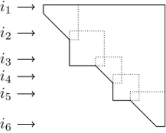
The projected counterpart Z = VHAV is highly structured. The submatrices
Z(ij :ij+1+ 1) for odd j, are of Hessenberg form, and the blocks corresponding to even j are of inverse Hessenberg plus diagonal form, with the perturbing diagonal equal to [0, ξij, . . . , ξij+1−1,0], which is a non-interrupted succession of finite poles
i1 i2 i3 i4 i5 i6
Fig. 3.1: Structure of the projected counterpart.
pre- and postpended with zero, except when ij = n. All the structured diagonal
blocks have thus an overlap of a 2×2 submatrix. Figure3.1 graphically depicts the positioning and overlap of the blocks. In the remainder of this article we will name such matrix anextended Hessenberg plus diagonal matrix. This is consistent with the nomenclature of extended Krylov spaces, which lack poles, and solely contain powers and inverses of A, implying thus an empty diagonal term. The matrix Z contains the recurrences for reconstructing the orthogonal column vectors of V which are, as mentioned before, tightly connected to orthogonal rational functions.
Using only infinite polesVHAV becomes Hessenberg; permitting only zero as a poleVHAV becomes of extended form as proved in [37]; in [34] it was demonstrated that allowing only finite poles results in an inverse Hessenberg plus diagonal matrix; here, however, a mixture of all these structures is allowed.
Inverse Eigenvalue Problem 3.1. Given a vector v = [v1, v2, . . . , vn]T
of weights, let Λ denote a diagonal matrix with as diagonal values the eigenvalues
λ1, λ2, . . . , λn. The vector of poles is ξ, and p the associated selection vector. The
problem to be solved is to efficiently compute the matrix VHΛV (and if required the
unitary matrix V) such that Ve1 = v/kvk2 and VHΛV is of extended Hessenberg
plus diagonal form, where D contains the poles ξ, and the extended Hessenberg ma-trix’ structure matches the position vectorp.
For finite poles only, this problem was solved in [33,34]. The introduction of infinite poles is as such slightly more general, but it must be stressed that with some nontrivial modifications the methods proposed in [33,34] are likely to deal with this problem as well. However, all the theoretical structure predicting proofs needed to be adapted as well to suit this more general setting. Moreover, the methodology and derivation of the algorithm in this article is entirely different, yet yielding the same outcome in case of only finite poles. These deductions do also allow a swift treatment of the more general inverse eigenvalue problem discussed in Section4.
3.2. Representation. Rather than storing the dense matrix VHΛV we will
factor it by its QR factorization and store the Q factor memory economical by de-composing it as a product of rotations. We will then operate on this rotational factorization.
The key-ingredient is the QR factorization; it is known that the unitaryQfactor in the QR factorization of a Hessenberg matrix comprises n−1 rotations [10,40]. More precisely, when Gi denotes the embedding of a rotator in the identity matrix,
having its effective part operating on rowsi and i+ 1, we have that a Hessenberg’s QR factorization can be written as H = G1G2G3. . . Gn−1R, in which the Q factor exhibits adescendingsequence of rotators. The inverse of a Hessenberg matrix, admits
a factorization of formGn−1Gn−2. . . G2G1R, where the factorization ofQis referred to as an ascending sequence of rotations; this can be proved easily by utilizing the techniques from Section3.3.
In general, the projected matrixZ associated to a rational Krylov space can be rewritten as ˜Z =Z−D, withDa diagonal matrix with precisely positioned poles on its diagonal, and ˜Zof extended Hessenberg form. The diagonal blocks in ˜Zare thus of Hessenberg or inverse Hessenberg form. Merging the QR factorizations of each of the diagonal blocks results in azigzag shaped ordering of the rotations, where ascending and descending sequences of rotations are taking turns.
Let us clarify by an example how the zigzag shape relates to the diagonal blocks. Take the selection vector as p= [i,i,i,f,f,f,f,i,i,i] associated to the vector of poles ξ. We have thus i1 = 1, i2 = 4, i3 = 8, i4 = 11. We get for starting vector v that
Krat
ξ,11(A,v) = {v, Av, A
2v, A3v, q4(A)−1v, q5(A)−1v, q6(A)−1v, q7(A)−1v, A4v, A5v,
A6v}. The associated projected counterpart ˜Z = Z−D obeys the structure visu-alized in Figure 3.2. The brackets with arrows denote rotations acting on the rows marked with the arrows. The crosses stand for possibly non-zero entries of the ma-trix. The three overlapping diagonal blocks are Hessenberg, inverse Hessenberg, and
× × × × × × × × × × × × × × × × × × × × × × × × × × × × × × × × × × × × × × × × × × × × × × × × × × × × × × × × × × × × × × × × × × × × × × × × × × × × × × × × × × × × × × = × × × × × × × × × × × × × × × × × × × × × × × × × × × × × × × × × × × × × × × × × × × × × × × × × × × × × × × × × × × × × × × × × × Fig. 3.2: QR factorization of an extended Hessenberg matrix.
again Hessenberg and they are emphasized and put in a square on the left. The right scheme reveals the graphical QR factorization of this matrix. To retrieve the QR factorization of the matrix ˜Z first the inverse Hessenberg blocks are factored with ascending sequences of rotations (counting from top to bottom we regard rotators 5 up to 8), next the Hessenberg blocks are factored by descending sequences of rotations (rotations 1 up to 4, and 9 up to 10).
A rigorous analysis of the ordering of the rotations furnishes us the following rule. Again each rotationGi is expected to operate on rowsiandi+ 1. Whenever theith
component pi of the selection vector pi equalsi, rotationGi is positioned to the left
of rotatorGi+1, valuepi=fsignifies that Gi is positioned to the right ofGi+1.
The structure we will try to retrieve in the inverse problem isZ =QR+D, with
D the diagonal with correctly positioned poles, andQR the QR factorization of the matrix ˜Z, withQfactored in rotations according to the selection vectorp.
3.3. Manipulating rotations. To work effortlessly with rotators, three basic operations are necessary: thefusion, theturnover, and thepass through action.
The fusion is the most elementary operation: Two successive rotations operating on identical rows can be united in a single rotation. Figure3.3(a)illustrates this.
The turnover action reshuffles three successive rotations: let F, G, H be three rotators affecting rows 1−2, 2−3, and 1−2 respectively. Then it is always possible
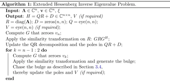
Algorithm 1:Extended Hessenberg Inverse Eigenvalue Problem. Input: Λ∈Cn,v∈Cn, ξ
Output: H=QR+D∈Cn×n,V (if required)
R= diag(Λ);D= zeros(n, n);Q= eye(n, n);
V = eye(n, n)(if required); ComputeGthat zeroesvn;
Apply the similarity transformation onR: GRGH;
Update the QR decomposition and the poles inQR+D; fork=n−1 : 2 do
ComputeGthat zeroesvk;
Apply the similarity transformation and generate the bulge; Chase the bulge as described in Section3.4,
thereby update the poles andV (if required); end
to refactor their product again in three rotations V, W, and X, operating now on rows 2−3, 1−2, and 2−3 so that F GH =V W X. Figure3.3(b) sheds some light on this change and reshuffle.
In the passing through operation we have a pattern of rotations gathered in the matrix ˜Q positioned to the right of an upper triangular matrix ˜R. Applying the leftmost rotation of ˜Qon the matrix ˜R(assume it acts on columnsiandi+ 1) creates a bulge in position (i+ 1, i). This bulge can be eliminated by a rotation on the left, acting on rows i and i+ 1. In this manner one can pass one by one the rotations in ˜Q through the upper triangular matrix and obtain a factorization QR, with Q’s shape identical to the one of ˜Q. The transition of all rotators on the right to the left is named the passing through operation. Of course a similar operation from left to right is also feasible. Figure3.3(c)depicts this.
= (a) Fusion = (b) Turnover × × × × × × × × × × × × × × × × × × × × × × × × × × × × × × = (c) Passing through
Fig. 3.3: Three basic operations on rotators.
3.4. Algorithmic solution. To tackle Problem3.1, we rely on the results from Section3.2 and do not compute the matrixVHΛV directly, but in factored form. A
pseudo-code of the algorithm is already depicted in Algorithm 1which is detailed in this section. We initiate the discussion by dealing with the cases with only infinite and only finite poles followed by a discussion on their integration.
3.4.1. Only poles at infinity. In this section the classical inverse eigenvalue problem to retrieve a Hessenberg matrix, given its eigenvalues and first vector of the unitary matrixV is considered. Though well-known [33,34], the description with rota-tors is new and enhances the comprehension of the generic algorithm. The algorithm
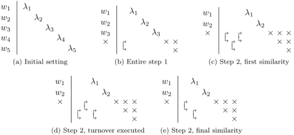
will be presented in a graphical manner, so we wish to retrieve the QR factorization of the Hessenberg matrix, consequently configured as a descending sequence of rotators. Figure3.4(a) depicts the initial setup for an example of dimension 5. A vertical line separates the vector of weights from the diagonal matrix of eigenvalues. Each step
i= 1, . . . , n−1 of the algorithm the (n−i+ 1)st element of the current weight vector is zeroed by a rotator acting on rowsn−i andn−i+ 1. This rotation determines the similarity to be executed on the associated matrix. Following this first similarity
i−1 other similarities (with rotations) are needed to remove the fill-in generated by the first similarity. As result we obtain the Hessenberg matrix in factored form.
Let us elude more on this by examining the 5×5 example. We assume that after a similarity the rotations on the right will always be passed through the upper triangular matrix immediately, making them thus appear on the left. Apart from the elements agreeing to those in the first figure, we will simply denote the matrix and weight elements by a×.
Figure3.4(b)depicts the result after annihilating the first weight, and performing the coupled similarity; the rotation positioned to the right of the matrix is first passed through the upper triangular (diagonal) matrix after which it is fused with the left positioned rotation. In Figure 3.4(c) the first similarity transformation of step 2 is executed; it is plainly visible that there is one additional rotation. To remove this rotation, first a turnover is needed resulting in Figure3.4(d). The outer left rotation determines the forthcoming similarity, such that the rotation itself vanishes after executing it; the similarity also introduces a rotator to the right, which after passing through the upper triangular matrix can be fused with the bottom rotator, providing us the result of step 2 in Figure3.4(e). Crucial in the latter similarity transformation, designed to chase the perturbing rotation, is that the zeros of the weight vector, after operating on the left, remain intact.
w1 λ1
w2 λ2
w3 λ3
w4 λ4
w5 λ5
(a) Initial setting
w1 λ1 w2 λ2 w3 λ3 × × × × (b) Entire step 1 w1 λ1 w2 λ2 × × × × × × ×
(c) Step 2, first similarity
w1 λ1 w2 λ2 × × × × × × ×
(d) Step 2, turnover executed
w1 λ1 w2 λ2 × × × × × × ×
(e) Step 2, final similarity
Fig. 3.4: Inverse eigenvalue problem having only poles at infinity (steps 1 and 2).
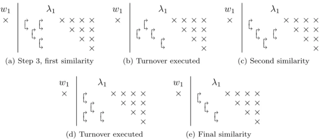
Figure3.5shows the flow of step 3. After the first similarity (Figure3.5(a)), again an undesired rotation is introduced. The turnover operation moves the unwanted rotation to the left and deposits it one row lower (Figure3.5(b)). A second similarity removes the outer left rotation and introduces another, still undesired rotation, on the right (Figure3.5(c)). Important is that the sparsity of the weight vector is maintained.
Another turnover brings this rotation to the left, once more positioned a row lower (Figure3.5(d)), which is removed next by a similarity (Figure3.5(e)).
w1 λ1 × × × × × × × × × × ×
(a) Step 3, first similarity
w1 λ1 × × × × × × × × × × × (b) Turnover executed w1 λ1 × × × × × × × × × × × (c) Second similarity w1 λ1 × × × × × × × × × × × (d) Turnover executed w1 λ1 × × × × × × × × × × ×
(e) Final similarity
Fig. 3.5: Inverse eigenvalue problem having only poles at infinity (step 3).
Continuing this procedure results in a Hessenberg matrix. Accumulating all ro-tations in a matrixVH. We have, by construction, thatVHΛV is of Hessenberg form andVHv=αkvk2e1, with|α|= 1, satisfying the requirements. The last step is the multiplication of the first column ofV withαand the first column and row ofH with
α. This does not effect the structure ofH and the problem is thus solved.
3.4.2. Only finite poles. A solution to this problem was already proposed in [33,34]. Though the approach presented in this section is theoretically equivalent, the onset and accordingly the entire description differs significantly. This differing approach provides additional insight and enables us to smoothly combine this and the algorithm of Section3.4.1to tackle the general setting.
The introduction of finite poles forces us to consider the more general factorization with the perturbing matrix D containing the poles. The basic idea is identical to Section 3.4.1. In each step the rotation determining the first similarity is designed to zero out an element in the weight vector followed by a succession of similarities to chase the remaining uninvited rotation. There are two crucial differences: whereas in the Hessenberg case the outer left rotators were selected to execute a similarity with, here the outer right ones will be taken. Another difference is the introduction of the poles, which require special handling. In the end we desire a factorization
QR+D, withQ factored as an ascending sequence of rotations,R upper triangular andD= diag(0, ξ1, . . . , ξn−1).
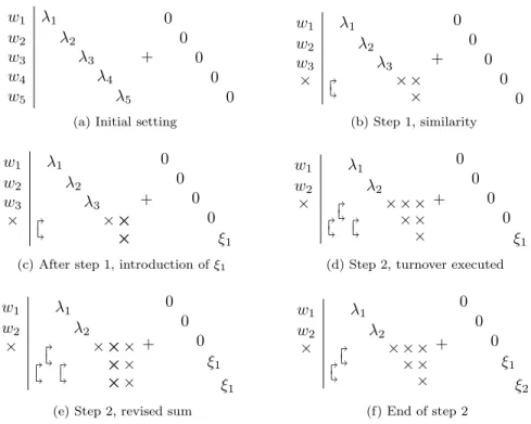
Figure3.6exemplifies the flow of the algorithm for a 5×5 matrix. Initially (Fig-ure3.6(a)) we start with the diagonal matrix Λ =Q0R0 plus a zero diagonal matrix
D0. The QR factorization of Λ will gradually be transformed to a QR factorization of desired form, whereas the matrixD0 will be modified to position the poles on the di-agonal. Executing the initial similarity of step 1 proceeds identical as in Section3.4.1
Figure 3.6(b). After this, one needs to fiddle with both terms to introduce the first pole in the zero diagonal matrix, the altered elements in the left term are typeset bold in Figure 3.6(c), and the first pole is introduced. After step 1 we have Q1R1+D1, whereQ1contains one rotator,R1is block diagonal, with one diagonal, and one upper triangular block, and D1 embodies the first pole. Step 2 kicks off as before. After
the similarity, passing through, and turnover we arrive at ˜Q2R˜2+D1, visualized in Figure 3.6(d). It is relevant to mention that the similarity transformation did not alter the diagonal matrixD1, its action was restricted to a part with equal diagonal values. Stated already before, the next similarity transformation, should be designed to remove the outer right rotator of ˜Q2. First, however, again a rewriting of the sum is required, as otherwise the similarity would destroy the requested diagonal structure of D1. The diagonal is altered to ˜D2 = diag(0,0,0, ξ1, ξ1), ensuing that a new QR factorization of the resulting modified left term ˜Q2R˜2−( ˜D2−D1) is preferred. We get
˜
Q2( ˜R2−Q˜H2( ˜D2−D1)) = ˜Q2Rˆ2, (3.2) where the term ˜QH2 ( ˜D2−D1) has only the three trailing elements in the penultimate column different from zero. Adding these elements to the upper triangular matrix ˜R2 gives us ˆR2, with a graphical representation of (3.2) in the left term of Figure3.6(e), displaying the affected elements in bold. There are now a troubling rotator and bulge simultaneously in the factorization ˜Q2Rˆ2. Fortunately both of them can be removed at once by a similarity. To pass the outer right rotator of ˜Q2, say ˆG, through ˆR2one applies it on ˆR2, providentially not creating a bulge, as it already exists. To remove this bulge one first passes this rotation to the right of the factorization: ˆGRˆ2= ˘R2G. This rotator G on the right now determines the next similarity transformation to be executed. The similarity does not destroy the structure of ˜D2 as the active part of the similarity operates on a scalar multiple of the identity in ˜D2. The newly appearing rotation GH on the left can be fused with the left rotation in ˜Q2, we
get GHQ˜2GˆH = Q
2 and Q2R˘2+ ˜D2. We end by modifying ˘R2, and ˜D2 to obtain
Q2R2+D2, withD2= diag(0,0,0, ξ1, ξ2) as depicted in Figure3.6(f).
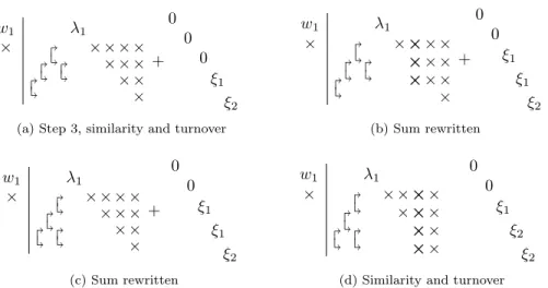
In Figure3.7step 3 is summarized. Besides the fact that more chasing steps are now required, the ideas remain unaltered. Figures3.7(a)and(b)show the result after the first similarity and turnover, and the result of modifying the diagonal of poles. The first similarity to chase the perturbations away and the following up rewriting of the sum are depicted in Figures3.7(b)and(c). Next another similarity and rewriting needs to be executed almost identical to Step 2.
Again it is easily verified that synthesizing all rotations executed results in a matrixVH, which satisfies the beforehand stated conditions.
Remark 3.2. The algorithm proposed in this section admits a slightly faster
im-plementation (see [33,34]) when one stores each of the diagonal inverse Hessenberg blocks appearing in the extended Hessenberg matrix. Each of these blocks must then be written as an outer product of two vectors. This compact writing allows the modifi-cations to the diagonal of poles in each chasing step to be performed more efficiently.
3.4.3. General case. It remains to integrate both the algorithms for finite and infinite poles by illustrating how to enforce the transitions from left to right and vice versa in the zigzag shape.
A study of both algorithms presented so far reveals, that once the chasing is initiated in the descending or ascending direction that all similarities are determined by either the outer left or outer right rotations. The remaining rotations are captured in the descending or ascending sequence. This statement holds for all except the final rotation (see Figures3.7(c)and3.7(d)) this rotation is not blocked by other rotations, and so one has the freedom to remove either the right or the left rotation.
Summarizing, in each step a new rotator on top is introduced along the descending or ascending line. Once reached the bottom (assume we can pass bends), one has the
w1 λ1 w2 λ2 w3 λ3 w4 λ4 w5 λ5 + 0 0 0 0 0 (a) Initial setting
w1 λ1 w2 λ2 w3 λ3 × × × × + 0 0 0 0 0 (b) Step 1, similarity w1 λ1 w2 λ2 w3 λ3 × ×× × + 0 0 0 0 ξ1 (c) After step 1, introduction ofξ1
w1 λ1 w2 λ2 × × × × × ×× + 0 0 0 0 ξ1 (d) Step 2, turnover executed
w1 λ1 w2 λ2 × ××× ×× ×× + 0 0 0 ξ1 ξ1 (e) Step 2, revised sum
w1 λ1 w2 λ2 × × × × × × × + 0 0 0 ξ1 ξ2 (f) End of step 2
Fig. 3.6: Inverse eigenvalue problem having only finite poles (steps 1 and 2).
liberty to remove either the left or right rotator and as such change the direction of the pattern. Each step (removal of an element in the weight vector) can thus be interpreted as pushing up the existing pattern of rotations, with flexibility of putting the new bottom rotation to the left or to the right of the existing ones. We will consecutively address three subproblems: how to pass a bend in the shape, how to carry out the transitions from finite to infinite poles and vice versa.
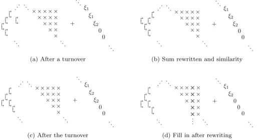
Passing a bend during chasing. We commence with tacklingthe bend problem. We assume that so far the chasing went smoothly and we arrived at the bend displayed in Figure 3.8(a) exhibiting part of a pattern with a bend. The matrix continues thus on the upper left and lower right corner. The vector of weights is no longer depicted. After the similarity shown in Figure3.8(a)the turnover is performed leading to Figure3.8(b). This figure illustrates that only one option, namely removal of the right rotator remains; recall, however, that before this point a descending sequence was encountered, so all similarities were determined by rotators positioned on the left of the sequence. From this point on we can proceed identically as in Section 3.4.2. To illustrate that this bend will move up one position Figures3.8(c) and 3.8(d) are included illustrating the modification of both terms before the similarity, and the result of the next similarity. Comparing Figures3.8(a)and3.8(d)plainly reveals the upward move of the pattern.
The other bend from finite to infinite is more involved. In Section3.4we deliber-ately did not specify the structure of the matrixD. Whereas one would tacitly assume the infinite poles to be linked to zeros inD, our representation does not allow an ef-ficient algorithmic design when allowing this. Instead we will repeat the previously
w1 λ1 × × × × × × × × × × × + 0 0 0 ξ1 ξ2 (a) Step 3, similarity and turnover
w1 λ1 × ××× × ×× × ×× × × + 0 0 ξ1 ξ1 ξ2 (b) Sum rewritten w1 λ1 × × × × × × × × × × × + 0 0 ξ1 ξ1 ξ2 (c) Sum rewritten w1 λ1 × × ××× ××× ×× ×× 0 0 ξ1 ξ2 ξ2 (d) Similarity and turnover
Fig. 3.7: Inverse eigenvalue problem having only finite poles (step 3).
... ... × × × × × × × × × × × × × × × .. . ... + ... 0 0 0 ξ1 ξ2 ... (a) Step 3, after a chasing similarity
... ... × × × × × × × × × × × × × × × .. . ... + ... 0 0 0 ξ1 ξ2 ... (b) After the turnover
... ... × × × × × ××× × ×× × ×× × × .. . ... + ... 0 0 ξ1 ξ1 ξ2 ... (c) Sum rewritten ... ... × × × × × × × × × × × × × × × .. . ... + ... 0 0 ξ1 ξ1 ξ2 ... (d) Similarity and turnover
Fig. 3.8: Passing a bend in the shape.
positioned pole inD as long as the actual associated pole remains infinite.
Let us clarify the problem and elegance of this solution further. Let us retain the straightforward idea of having infinite poles linked to zeros inD. Assume at a certain point we have completed a turnover and we arrive in Figure3.9(a). Rewriting of the sum (modifying the secondξ1into ξ2) followed by a similarity give us Figure3.9(b). After the next turnover, in which we pass the bend (Figure 3.9(c)) the problems become clear. To modify the trailing ξ2 in 0 a rewriting of the sum is required, however, this would create a downward spike of undesired non-zeros up to the next bend. This spike cannot be removed, so we have to prevent it from the start by, e.g., keeping the poleξ2instead of trying to make it zero. Since the vectors{v,(A−σI)v}
span the same space as{v, Av}, keeping the poleξ2does not affect the infinite poles. Let us see what happens if ξ2 were repeated. We proceed almost identical, as we
.. . ... × × × × × × × × × × × × × × × ... ... + ... ξ1 ξ1 ξ2 0 0 ... (a) After a turnover
.. . ... × × × × × × × × × × × × × × × ... ... + ... ξ1 ξ2 ξ2 0 0 ... (b) Sum rewritten and similarity
.. . ... × × × × × × × × × × × × × × × ... ... + ... ξ1 ξ2 ξ2 0 0 ... (c) After the turnover
.. . ... × × ××× × ××× ××× ×× ×× ... ... ... + ... ξ1 ξ2 0 0 0 ... (d) Fill in after rewriting
Fig. 3.9: Possible problems in passing a bend from finite to infinite poles.
assume again at a certain point to have completed a turnover (Figure3.9(a)). Again the sum is modified and followed by a similarity (Figure3.9(b)). The last two Figures, Figures 3.10(c)and (d), show again that the pattern moves up one position and no special rewriting of the sum is required anymore. We can retain our efficient QR representation. .. . ... × × × × × × × × × × × × × × × ... ... + ... ξ1 ξ1 ξ2 ξ2 ξ2 ...
(a) After a turnover
.. . ... × × × × × × × × × × × × × × × ... ... + ... ξ1 ξ2 ξ2 ξ2 ξ2 ... (b) Sum rewritten and similarity
.. . ... × × × × × × × × × × × × × × × ... ... + ... ξ1 ξ2 ξ2 ξ2 ξ2 ... (c) After the bend turnover
.. . ... × × × × × × × × × × × × × × × ... ... + ... ξ1 ξ2 ξ2 ξ2 ξ2 ...
(d) After the similarity
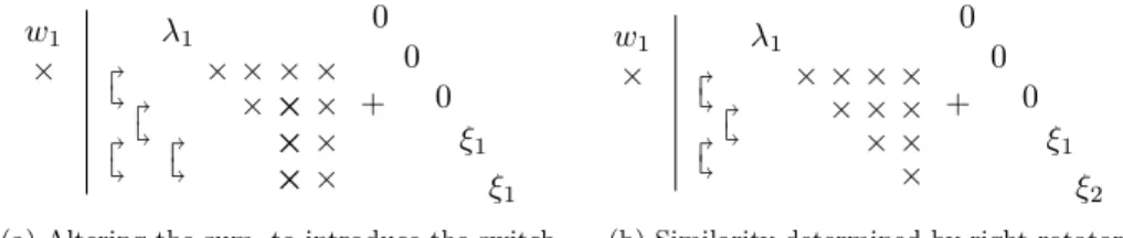
Interchanging the pole type: from infinite to finite and vice versa. Next we illus-trate the transition from infinite to finite poles, on a 5×5 example where the first two rotations were put descendingly. Suppose we arrived at the situation depicted in Figure3.4(e), and then after some chasing steps we arrive in Figure3.5(d). To con-tinue the design of a descending sequence one just follows Figure3.5. Here, however we desire to change the direction. Before the similarity the diagonal matrix (zero in this case) needs to be introduced. Figure3.11(a) depicts the novel situation. After the similarity determined by the right rotator and some rewriting to introduce pole
ξ2 we get Figure 3.11(b). The onset is now made and a combination of the chasing
w1 λ1 × × × × × ××× ×× ×× + 0 0 0 ξ1 ξ1 (a) Altering the sum, to introduce the switch
w1 λ1 × × × × × × × × × × × + 0 0 0 ξ1 ξ2 (b) Similarity determined by right rotator
Fig. 3.11: Transition from infinite to finite poles.
in the descending sense, passing a bend, and chasing in the ascending sense, one can pursue the introduction of new rotations to prolong the current ascending sequence.
The transition fromfinite to infinitepoles acts in accordance with the previously described transition. The details are left to the reader, who should not forgot the repeat the final finite pole for being able to effectively pass bends.
Integrating Sections 3.4.2 and 3.4.1 with the last-mentioned transition actions bears us the desired algorithm to solve the inverse eigenvalue problem.
3.5. Particular configurations of eigenvalues. In this article we refrain from adapting and optimizing our algorithm for particular configurations of eigenvalues. We do present the effect on the matrix structure for some classics below. More general cases, e.g., eigenvalues on curves, can be found in [13,19,21] and the references therein. All eigenvalues located on the real line implies symmetry, i.e.,ZH=VHΛHV =
VHΛV =Z. Hence the Hessenberg blocks become tridiagonal and the inverse
Hes-senberg plus diagonal parts become semiseparable plus diagonal blocks. Since we have Z = VHΛV and ZH = VHΛHV = Z. It is evident that exploitation of this
structure is compulsory for the development of an efficient algorithm. If we choose the eigenvalues on an arbitrary line in the complex plane we loose the symmetry but still get a tridiagonal matrix. Since there is a Λe ⊂ R with Λ = αΛ +e βI and the
sparsity pattern ofZ, written as
Z =VHΛV =αVHΛeV +βVHV,
is not affected by multiplying with αor by shifting with β. Also the semiseparable structure of the upper and lower triangular parts is not affected.
All eigenvalues situated on the unit circle, thus of modulus 1, signifies that the associated matrix is unitary. A unitary Hessenberg matrix has the attractive property that his lower triangular part is sparse and its upper triangular part is rank structured. Allowing only infinite and zero poles one can prove that the associated matrix of recurrences can be represented by solely a zigzag sequence of rotations. Considering
the dense matrix, one acquires alternating and overlapping diagonal blocks of upper Hessenberg and lower Hessenberg form.
If all eigenvalues lie on an arbitrary circle, then we can again shift and scale the problem so that the eigenvalues lie on the unit circle. The scaling does not change the rank structure nor the sparsity pattern of the resulting matrix. But the shifting changes the diagonal and soZhas only a rank structure in the strict lower resp. upper triangular part.
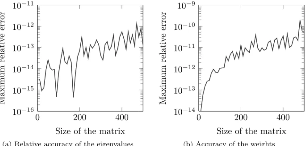
3.6. Numerical experiments. We have tested our algorithm with sets of ran-dom eigenvalues in the complex plane (λ=rand(n,1)+i∗rand(n,1)), random complex weights (generated identical to the eigenvalues) and a random selection vector, where we change from infinite to finite and vice versa with a probability of 30%. We ran for each matrix dimension five tests. The maximum relative error is the maximum over all five tests. After having computed the projected counterpart, we recomputed its eigenvalue decomposition providing us eigenvalues ˜λi and weights ˜wi. For each run
the relative error on the eigenvalues was computed as maxi|˜λi−λi|/|λi|,the relative
error of the weights was computed identically.
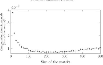
Figures 3.12(a) and 3.12(b) show that the computed matrix have the wanted eigenvalues and the wanted weights. Figure3.13shows that the algorithm is of cubic complexity. The computation time is averaged over the five tests. The experiments were conducted inMatlabon an IntelRXeonRCPU E5645 with 2.40 GHz.
0 200 400 10−16 10−15 10−14 10−13 10−12 10−11
Size of the matrix
Maxim
um
relativ
e
error
(a) Relative accuracy of the eigenvalues
0 200 400 10−14 10−13 10−12 10−11 10−10 10−9
Size of the matrix
Maxim
um
relativ
e
error
(b) Accuracy of the weights
Fig. 3.12: Relative accuracy.
4. The inverse eigenvalue problem for extended tridiagonal matrices. In this section we will reconstruct the projected counterpart, linked to the nonsym-metric Lanczos algorithm, with predetermined poles, eigenvalues and weights. This projected counterpart contains the recurrences between biorthogonal sequences of ra-tional functions.
In Section4.1we prove that the projected counterpart will be of extended tridiag-onal form. A compact factorization of this matrix is essential for the development of an efficient algorithm and is presented in Section4.2. As we loosen the orthonormality constraint on the basis vectors, we cannot rely solely on unitary operations anymore
0 100 200 300 400 500 1 2 3 4 ·10 −5
Size of the matrix
Computation time in sec onds (Size of the matri x) 3
Fig. 3.13: Computational complexity.
and also eliminators will be used. Section4.3discusses the essential operations for the algorithm design. In Section 4.4 the algorithm is presented, followed by Numerical experiments in Section4.5.
4.1. Induced matrix structure & Problem formulation. Detailed knowl-edge of the structure of the matrix capturing the recurrence coefficients is essential when trying to reconstruct it. To derive this structure we draw heavily from Sec-tion3.1.
Given two vectors of poles ξ = [ξ1, ξ2, . . . , ξn], and χ = [χ1, χ2, . . . , χn] with
ξi, χi∈ {0,∞}, fori= 1, . . . , n, the following two extended Krylov spaces are
consid-eredKrat
ξ,`(A,v) andKratχ,`(AH,w) for two vectors of weigths, and under the additional
assumption thatwHv= 1. In this article we exclude pure finite poles.
The upcoming deductions differ significantly from the conventional manner of iteratively constructing the basesW andV. This alternative matrix view enables us, however, to reuse the results from Section 3.1for deducing the structure of WHAV
swiftly and comprehensibly. Assume, we have constructed ˆV and ˆW as orthogonal bases for both extended Krylov spaces. We know that ˆK and ˆZ satisfy
AVˆ = ˆVZˆ and AHWˆ = ˆWKˆ (4.1) obeying the extended Hessenberg structure presented in Section 3.1. Hence both matrices ˆKand ˆZhave thus alternating and overlapping diagonal blocks of Hessenberg and inverse Hessenberg form, imposed by the setting of the poles inξandχ.
The actual desired basesV andWneed to span the same intermediately generated Krylov spaces as ˆV and ˆW and must be biorthogonalWHV =I. These matrices can
be retrieved asV = ˆV(DU)−1 andWH =L−1WˆH, where ˆWHVˆ =LDU is an LDU decomposition1, which meansLis unit lower triangular,U unit upper triangular, and
D diagonal. Plugging this decomposition in (4.1), we have that
AV =AVˆ(DU)−1= ˆV(DU)−1(DU) ˆZ(DU)−1=V (DU) ˆZ(DU)−1=V Z, AHW =AHW Lˆ −H= ˆW L−HLHKLˆ −H=W(LHKLˆ −H) =W K.
1Obviously an LDU factorization need not exist. In this case this procedure, just as the classical
We are fortunate now as multiplications with upper triangular matrices to the left and to the right of a matrix do not have an impact on the lower triangular structure. As a result ˆZ and Z, and ˆK and K share their structure, i.e., the Hessenberg and diagonally perturbed inverse Hessenberg blocks are positioned identically, even the diagonal elements remain untouched. Moreover, by construction we have now that
Z=KHand as such we have the structure for the lower as well as the upper triangular part.
Whereas in the original case as in Section3structure (letting slip the configuration of eigenvalues, see Section 3.5) was only imposed below the diagonal, we now have structure above as well as below the diagonal. Note, however, that these two structures are unrelated. Both are only and strictly connected to the individual independently chosen Krylov spaces. Figure 4.1 reveals a possible configuration, where obviously upper and lower triangular structures are uncorrelated. It might seem unnatural that
Fig. 4.1: Possible structure in the nonsymmetric Lanczos case.
the upper part apparently has two successive perturbed inverse Hessenberg blocks. Taking into account an overlap of 2×2 blocks, this can be enforced by a single infinite pole in the sequence. To match our previous nomenclature, though slightly misleading as the matrix is not tridiagonal, we will address this type of matrix anyway as anextended tridiagonal matrix2.
Inverse Eigenvalue Problem 4.1. Consider the vectorsw= [w1, w2, . . . , wn]T
andv= [v1, v2, . . . , vn]T containing the weights and let wHv= 1. Let Λbe the
diag-onal matrix of eigenvalues. The poles for the Krylov spaces withAandAH are stored in the vectorsξandχrespectively3. The inverse problem involves the construction of the matrix WHΛW−H =WHΛV =V−1ΛV (and if desired the matrices V andW) satisfying the structural constraints as imposed by the vectors of poles as presented in Section 4.1. Moreover the two matricesV andW have their first vectors equaling
v and w, up to a scalar, and they are biorthogonal. This means We1 = ωw and
Ve1=νv, withω andν two scalars; the biorthogonality impliesWHV = 1.
The algorithm presented in this article to solve this problem can suffer from nu-merical instabilities. Furthermore, like in the classical nonsymmetric Lanczos, break-downs and near breakbreak-downs can occur. Look-ahead is a possible solution; this is the subject of future research.
4.2. Representation. In the first inverse eigenvalue problem, most of the op-erations involved manipulating rotations. As we step away from unitarity here, we must also refrain from relying only on manipulations involving rotators.
2Every extended tridiagonal matrix is quasiseparable, but the other statement does not hold: a
quasiseparable matrix is not necessarily of extended tridiagonal form.
3The problem and solution presented here are not yet capable of dealing with finite, nonzero
Instead we will use nowGaussian elimination matrices zeroing only one element at once, and also changing only one row or column in doing so. To have a short name consistent with rotator, we will address these matrices as eliminators. Contrary to the rotators, there are two types of eliminators having either
1 0 × 1 or 1 × 0 1
embedded in the identity matrix, named lower resp. upper eliminators as they are lower resp. upper triangular. As before we will use a bracket to represent such an eliminator. This bracket will only have one arrow pointing to the row containing the entry×. Graphically we thus get
d= 1 × 1 and b= 1 × 1 .
When executing an eliminator-matrix product the bracket also allows another inter-pretation: in the resulting matrix the row pointed to will change by adding a multiple of the row marked by the bracket’s other leg to it. Again only eliminators acting on successive rows are allowed, this means that one can only add a multiple of row i
to row i+ 1 or rowi−1 when executing an eliminator-matrix product. The lower and upper triangular eliminators are notated as Li and Ui respectively, where thei
indicates the row affected under the multiplication, this means that onlyL2, . . . , Ln
andU1, . . . , Un−1 are used.
Furthermore, we will no longer represent our matrix by the QR factorization consisting of a single zigzag shaped series of rotations and an upper triangular. We replace it by an LDU factorization, where both LandU are zigzag shaped products ofn−1 eliminators: L=Lp(2)· · ·Lp(n)andU =Uq(1)· · ·Uq(n−1), wherepandq are permutations in{2, . . . , n}and{1, . . . , n−1}respectively. The matrixDis diagonal. For instance, letT be a tridiagonal matrix with LDU factorizationT =LDU. One can show that the matricesL andU can be factored in a product of eliminators like
1 × 1 × 1 × 1 × 1 D 1 × 1 × 1 × 1 × 1 = d d d d D b b b b . (4.2)
Considering the case where both Krylov spaces only contain finite poles (i.e., 0 in this setting), the LDU factorization of the projected counterpart would have a factorization of the form
d d d d D b b b b . (4.3)
For an existence proof of such a factorization we refer to [38], where it is proved that both the L and U factors in an LDU factorization inherit the lower respectively upper triangular structure of the original matrix. The L andU factors can then be factored as products of essentially 2×2 lower and upper triangular matrices, which are elimination matrices.
So, in general we need to retrieve factorizations for example of the form d d d d d D b b b b b , (4.4)
where both theLandUfactor are independently built as a zigzag shape of respectively lower and upper eliminators. We will not go into the details, but the ordering of each individual sequence is bond to a selection vector: one selection vector for the lower part linked toξand one for the upper part related toχ.
4.3. Manipulating eliminators. We will again manipulate matrices in a fac-tored form. Therefore we need additional operations for dealing with eliminators, just like in Subsection 3.3. The two most important ingredients are the LDU and UDL factorization of a 2×2 matrix, graphically depicted as
× × × × = d × × b and × × × × = b × × d .
We also need to fuse eliminators:
d d = d , b b = b .
There are three slightly different settings in which we have to pass scalars through eliminators. In the next equations, the factorαstands in fact for a diagonal matrix equal to the identity, having only one diagonal entry replaced by α. Graphically the passing through reads as
α d
= d α , α b = b α , d
α = d α , and α b = b α .
Bare in mind that the eliminators involved in these equalities generally change as well. Eliminators also admit turnover operations just like the rotations4
d d d = d d d and b b b = b b b .
The eliminators have much more flexibility to rearrange their positions compared with rotations. Of course we can change the ordering of eliminators acting on different rows. But we also can do the following swaps, interchanging the position of two eliminators of which one is upper and the other is a lower eliminator. Note that the eliminators are not modified:
b d = d b and d b = d b .
4We remark that this turnover is almost always possible, see [5], possible breakdowns are inherent
Algorithm 2:Extended Tridiagonal Inverse Eigenvalue Problem. Input: Λ∈Cn,v,w∈Cn,ξ
Output: Z=LDU ∈Cn×n,V, W (if required)
Z= diag(Λ);D= zeros(n, n);Q= eye(n, n);
V =W = eye(n, n)(if required); ComputeGV that zeroesv
n and computeGW that zeroeswn;
BiorthogonalizeGV andGW;
Apply the similarity transformation onZ, and update its LDU decomposition; fork=n−1 : 2 do
ComputeGV that zeroesv
k and computeGW that zeroeswk;
BiorthogonalizeGV andGW;
Apply the similarity transformation and generate the bulge; Chase the bulge according to the four cases in Fig.4.4, thereby updateV andW (if required);
end
For a swapping of the following particular configuration
d
b and d b
we have to form the product of both matrices and compute the LDU or UDL factor-ization. We cannot circumvent in this case the introduction of an additional diagonal matrix, which by the passing through can be moved to the outer left or outer right.
These swap operations allow us topush lower eliminatorsthrough a sequence of upper eliminators without altering the rows they act on, the same holds forpushing
upper eliminators through sequences of lower eliminators. For example, it is easily verified that (ignore the possible introduction of an extra diagonal)
b d b b = d b b b .
It is unnecessary to provide proofs for the operations provided in this section: one can easily show how they are computed by forming the 2×2 resp. 3×3 matrices. We note, however, that some of these operations can potentially be unstable.
4.4. Algorithmic solution. This section elaborates on Algorithm 2 to solve Problem4.1and is split in several subsections separating zero, infinite, and mixed pole combinations. Again, instead of operating on the dense matrix directly we represent it in factored form as presented in Section4.2.
Before initiating our discussion, we would like to recall that in the previous section we always used unitary transformations and thus the Hermitian conjugate and the inverse coincide. Here, however, we recurrently use triangular matrices, either upper or lower. The Hermitian conjugate of such matrices makes upper become lower and lower become upper triangular; the inverse on the contrary does not affect the upper and lower structural constraint. We make an effort to overcome any ambiguity as much as possible.
Whereas in Section3we confined ourselves to unitary transformations, this must be loosened here. We will enforce the first columns of W and V to be w and v by combining unitary, upper-, and lower triangular operations to carry out dedicated tasks destroying neither the first columns of W and V nor the desired structure of the matrix of recurrences. In general we name any essentially 2×2 matrix embedded in the identity and acting on two successive rows or columns a core transformation, which can be a rotator, an eliminator, or a combination.
More precisely, each core transformation to be executed has specified tasks. In each step the first two core transformations executed (left and right) must annihilate elements in the weight vector and must be biorthogonal. The core transformations applied on both sides in the chasing procedure must annihilate bulges and secondly not destroy the biorthogonality. Each core transform encompasses thus two tasks: zero creation and biorthogonality enforcement. To easily achieve this, we will decompose each core transform in a QR or QL decomposition. The unitary factor will impose the zero structure, the upper triangular or lower triangular factors will enforce the biorthogonality;Rfor the first (left and right) transforms,L in the chasing part.
4.4.1. Only poles at infinity. We initiate our description with the simplest case, namely two classical Krylov spaces. The generic outcome should thus be a nonsymmetric tridiagonal matrix. For this setting it is instructive to first describe the flow of the algorithm by operating directly on the dense matrix. In Section4.4.2
we translate this to the new factorized representation.
Figure 4.2(a) shows the initial setting. The matrix Z0 = Λ is enclosed by the two weight vectors: w0 =w on its left, and v0 =v on top. The vector v is inten-tionally blessed with the conjugate such that the operations applied on the weight vectors can also be applied immediately on the inner matrixZ0. In the first step, the weights w5 and v5 are annihilated by a left (GW0,4)H and a right GV0,4 rotation. The subscripts (i, j) in the notation read as follows: i denotes the step, where each step annihilates one element in both weight vectors; andj points to the rows/columnsj
and j+ 1 affected by the operation. The meaning of the superscripts is clear from the context. The matrices Zi denote the outcomes after each step. As a result
we get (GW
0,4)−1w0 = (G0W,4)Hw0 = ˜w0 and (GV0,4)−1v0 = (GV0,4)Hv0 = ˜v0, both having as final element zero. The result of applying these transformations on Z0: (GW
0,4)HZ0GV0,4 as well is depicted in Figure 4.2(b). To complete the first step it re-mains to enforce biorthogonality betweenGW0,4andGV0,4, this is achieved by assigning
W0=GW0,4(L0,4D0,4)−HandV0=GV0,4U −1
0,4, where (GW0,4)HGV0,4=L0,4D0,4U0,4is an LDU decomposition. IndeedW0HV0= (L0,4D0,4)−1(GW0,4)
HGV 0,4U −1 0,4 =Iand we get Z1 =W0HZ0V0= (L0,4D0,4)−1(GW0,4)HZ0GV0,4U −1
0,4. The matricesWi andVj gather
all transformations executed in a single step. Fortunately also the biorthogonality reinforcement does not destroy the created zeros in the weight vectors as
W0−1w0= (L0,4D0,4)H(GW0,4)−1w0= (L0,4D0,4)Hw˜0=w1
V0−1v0=U0,4(GV0,4)−1v0=U0,4v˜0=v1,
both having the trailing vector element zero since (L0,4D0,4)H and U0,4 are upper triangular. Figure4.2(b)shows the result after the entire first step.
Figure 4.2(c) shows the result after the first tasks in step 2. We see –neglect the core transformations for a moment– the outcome of annihilating elements in the weight vectors as well as the biorthogonality reinforcement. Zeroing an element in w1 and v1 is achieved by transformationsGW1,3 and GV1,3, we get (GW1,3)−1w1 =
(GW
1,3)Hw1 = ˜w1 and (GV1,3)−1v1 = (GV1,3)Hv1 = ˜v1, having the penultimate and final element zero. Again, as in step 1, we update the transformation matrices to get them biorthogonal as follows ˜W1 = GW1,3(L1,3D1,3)−H and ˜V1 = GV1,3U
−1 1,3, where (GW
1,3)HGV1,3 = L1,3D1,3U1,3 is again an LDU decomposition. Executing ˜
WH
1 Z1V˜1 creates, however, unwanted elements in the second sub- and second su-perdiagonal. Next we need to remove these undesired nonzero elements in the outer corners of the lower right dense 3×3 block to revert back to the tridiagonal struc-ture. This removal is referred to as the chasing procedure. Executing the two rotations depicted in Figure 4.2(c) accomplishes this, name them GW1,4 and GV1,4. We have now ˜Z1 = (GW1,4)
HW˜H
1 Z1V˜1GV1,4 of tridiagonal form as in Figure 4.2(d). Unfortunately, we cannot apply the previous trick to reenforce the biorthogonality as utilizing the factors of the LDU decomposition would destroy the just reestab-lished tridiagonal structure. Using, however, the UDL decomposition, with U up-per,D diagonal, andL lower triangular and lettingW1= ˜W1GW1,4(U1,4D1,4)−H and
V1 = ˜V1GV1,4L−
H
1,4 where ( ˜W1G1W,4)H ( ˜V1GV1,4) =U1,4D1,4L1,4 we get the biorthogo-nality asW1HV1= (U1,4D1,4)−1( ˜W1GW1,4) H( ˜V 1GV1,4)L −1 1,4=I. Moreover, by consider-ingZ2=W1HZ1V1= (U1,4D1,4)−1( ˜W1GW1,4)HZ0( ˜V1GV1,4)L −1 1,4= (U1,4D1,4)−1Z˜1L−11,4, we see that the matrixZ2 must be of tridiagonal form, as (U1,4D1,4)−1 is upper
tri-angular,L−11,4is lower triangular and they only act on the last two rows and columns. In fact, one has everything now to run the algorithm to the end. Every similarity is executed in the same manner. In step 3, however, the biorthogonality enforcement in the chasing step will introduce new bulges, positioned lower, which in turn need to be removed by another chase step. In general step i requires i-1 chasing steps to remove the bulges and arrive at the tridiagonal form. For completeness, step 3 and step 4 are visualized in Figures4.2(e)and 4.2(f).
To summarize, each core transformation used in this procedure, is decomposed as either a unitary–upper triangular, or unitary–lower triangular product. The LDU decomposition is used for imposing biorthogonality while retaining the zero structure of the weight vectors. The UDL decomposition is needed for the biorthogonality en-forcement in the chasing procedure. This subtle difference between using the LDU and UDL factorization is due to the difference between inverting and taking the con-jugate transpose, namely Wi−1 and Vi−1 need to be applied on the weight vectors, whereasWiH andVi are applied on the matrixZi.
4.4.2. Only poles at infinity – factorized representation. Let us now re-consider the previous algorithm, but work directly on the factored representation of the tridiagonal matrix as in (4.2). This will help us to describe the forthcoming algo-rithm dealing with finite and infinite poles. The main difference between this and the Arnoldi algorithm from Section3.4is the appearance of a whole bunch of intermedi-ate swappings of lower and upper triangular eliminators. These swaps are essential to repositioning the eliminators so that all lower and upper eliminators are gathered allowing us to carry out turnovers and fusions.
Again, we will deal with a 5×5 example, initially looking as in Figure4.3(a). First we compute the rotationsGW0,4andG0V,4that annihilatew5andv5. To biorthogonalize them we compute the LDU factorization of (GW
0,44)HGV0,4and updateGW0,4andGV0,4 ac-cordingly. The essentially 2×2 matricesW0andV0contain all the information to com-plete the first step. As we wish to store a factored representation as in (4.2), we write
W0 and V0 as LDU decompositions and get a matrix product like in Figure4.3(b), whereW0=LW0,4DW0,4U0W,4 andV1=LV0,4DV0,4U0V,4. We can reorganize the lower and