The Impact of Competition on Technology Adoption: An Apples-to-PCs Analysis

The Impact of Competition on Technology Adoption:

An Apples-to-PCs Analysis

∗

Adam Copeland

and Adam Hale Shapiro

August 4, 2010

Abstract

We study the effect of market structure on a firm’s decision to adopt a new tech-nology in the personal computer industry. This industry is unusual because there exists two horizontally segmented retail markets with different degrees of compe-tition: the IBM compatible (or “PC”) platform and the Apple platform. We first document that relative to Apple, producers of PCs have more frequent technology adoption, shorter product cycles, and steeper price declines over the product cycle. We then develop a parsimonious vintage-capital model which matches prices and sales of PC and Apple products. The model predicts that competition is the key driver of the rate at which technology is adopted.

Key words: innovation, market structure, computers

JEL classification: D40, L10, L63, O30

∗_{We thank Ana Aizcorbe, Olivier Armantier, Steve Berry, Ben Bridgman, Phil Haile, Kyle Hood,}

Bronwyn Hall, David Mowery, Matt Osborne, Ariel Pakes, Jeff Prince and Dave Rapson for their comments and suggestions. This research was conducted under the BEA’s mission to better understand how firms value introducing new products into the market and their incentive to innovate. The views expressed here are those of the authors and do not necessarily reflect the position of the Bureau of Economic Analysis, the U.S. Department of Commerce, the Federal Reserve Bank of New York, or the Federal Reserve System.

†_{Federal Reserve Bank of New York; e-mail:[email protected];} ‡_{Bureau of Economic Analysis; e-mail: [email protected]}

1

Introduction

A multitude of industries consist of downstream firms which adopt technological innovations developed by upstream manufacturers. Cameras, cell phones, stereos, and personal computers (PCs) are examples of such goods which can be thought of as an

assembly of individual innovative components.1 _{Firms producing these types of consumer}

goods are “technology adopters” in the sense that they choose whether or not to adopt a new technology, but the technological limit, or frontier technology, is dictated by upstream firms.

In this paper, we analyze the relationship between market structure and technological adoption in the personal computer industry. Our work makes two contributions. First, we provide a descriptive analysis of the industry, measuring rates of technology adoption, consumer income distributions, as well as prices and sales over a typical computer’s life cycle. Second, we use a vintage-capital model to quantify the importance of market structure on determining the outcomes of these variables.

Similar to many other technological industries, the personal computer market is one in which adoptions are extraordinarily frequent and new products almost always incor-porate new technology advances. Unlike most industries, however, an important feature of the personal computer industry is the existence of two segmented retail markets. The industry is divided between two platforms: the IBM compatible platform (or simply

the “PC”) and the Apple platform.2 _{While there are many differences between these}

platforms, the largest difference is arguably their operating systems; PCs run on

Mi-crosoft Windows while Apples run on Mac OS.3 _{The horizontal differentiation between}

PCs and Apple therefore segments the retail market in the sense that consumers of PCs

1_{The central processing unit (CPU), for instance, which is a key component of many of these products,}

is in many cases produced by chip manufacturers.

2_{For a general overview of the history of competing platforms see Bresnahan and Greenstein (1999).}

Given the evolution of this industry, the IBM compatible platform is also referred to as the Wintel platform, a label that alludes to the Windows operating system and Intel processor combination used by the vast majority of these computers.

3_{Stavins (1995) refers to this type of platform differentiation as horizontal differences in the order of}

quality. This is in contrast to to vertical differences (e.g. speed and memory) along a certain platform line.

do not consider Apple products as close substitutes and vice-versa.4 _{This segmentation} is crucial for our analysis, because there are many firms that manufacture PCs, while only one firm that manufactures Apple computers. Thus, one can think of Apple as having a great deal of market power because it has no close vertical substitutes by other computer manufacturers for any specific product line (e.g. 15-inch notebook computers). Such segmentation allows us to compare and contrast the technology adoption decisions for a computer manufacturer in a competitive versus monopolistic market.

Our paper builds on the historical literature commencing with Schumpeter (1934,1942), and later Arrow, who examined the impact of competition on research and development

(R&D) activity. There has been an ongoing line of research dedicated to the topic.5

Schumpeter argued that since a monopolist gets to reap all of the rewards of a techno-logical innovation it has a higher incentive to undertake R&D costs than a competitive firm. Arrow described a scenario where a competitive firm has a higher incentive to undertake R&D since innovation provides a tool to escape competition by differentiat-ing itself from its competitors. Whereas these studies were referrdifferentiat-ing to industries in which R&D is undertaken directly by the innovating firm, their question addressing the impact of competition on incentives for innovation is relevant to technological-adopting firms. Similar to firms undertaking R&D, technological adopters incur large sunk costs, including marketing, assembly, and the establishment of retail channels. Thus, these firms must also weigh the cost against the marginal profit of undertaking an innovative investment.

Using NPD Group scanner data from 2001 to 2009, we compute various statistics on the rate of product entry across firms. Furthermore, we present evidence that new computers embody new technologies, making them higher quality products relative to the existing set of comparable computers. A striking feature of the data is that they

4_{Bresnahan, Stern and Trajtenberg (1997) differentiate the source of transitory market power in}

the personal computer industry between frontier (vertical quality) and brand (horizontal quality). The authors find that the effects of competition were confined to substitution clusters, and that brand differentiation provides protection from competition along similar vertical dimensions.

5_{See Aghion, Harris, Howitt, Vickers (2001), Aghion, Bloom, Blundell, Griffith, Howitt (2005),}

Aghion, Blundell, Griffith, Howitt, Prantle (2009), Aghion and Howitt (1992), Biesebroeck and Hashmi (2009), Dasgupta and Stiglitz (1980), Gilbert and Newbery (1982), and Goettler and Gordon (2009).

unequivocally show that Apple is slower at technological adoption than the other PC manufacturers. Overall, our data show that PC manufacturers are introducing signifi-cantly more products with shorter life spans relative to Apple. Thus, the data suggest that a more competitive market structure acts to increase the rate at which firms adopt new technological innovations.

The difference in adoption decisions between PC manufacturers and Apple is likely to be a function of many factors. To better understand the importance of market structure in explaining the differences in the rates of adoption across Apples and PCs, we use a parsimonious vintage-capital model. Our strategy is to parameterize the model to match the stylized facts on technology adoption, pricing, sales, and consumer income distributions for PCs, the market in which many firms compete. We then use the model to make an out-of-sample prediction on technology adoption, prices, sales, and consumer income given a monopolistic market structure. Surprisingly, the model’s predictions closely match the stylized facts for Apple computers. Essentially, keeping preferences and technology fixed, and only changing market structure, the model is able to match the different stylized facts for both PC and Apple computers. Consequently, a main result of the paper is that market structure plays a major influence on the rate of technological adoption in the market for personal computers.

Importantly, the model provides insight as to how and why the competitive market

structure generates higher rates of technology adoption. On the demand side, we use the quality-ladder framework of Shaked and Sutton (1982, 1983), henceforth, SS. On the

supply side, firms offer computers of different vintages and compete in price.6 _Computer

manufacturers face a constant marginal cost and pay a sunk cost to update their prod-uct. Within this environment, the introduction of a new, higher quality computer places enormous pricing pressure on all existing computers. Indeed, while the highest quality computer captures a large market share, simultaneously charging a large markup, lower quality computers capture a relatively small portion of the market and charge minimal markups. Hence, once a firm’s computer has been displaced as the highest-quality prod-uct, its per-period profits are fairly small. Given the rapid availability of new technology,

6_{Our supply-side model is similar to Aizcorbe and Kortum (2005), who use a vintage-capital model}

to analyze pricing and production in the semiconductor industry. Besides focus, our papers differ in our incorporation of consumer heterogeneity.

the model predicts steep falls in price, sales, and consequently profits, over a computer’s product cycle. This “market-specific” obsolescence generates a significant premium on having the highest-quality product in the market. Following the reasoning originally posed by Arrow and more currently by Aghion et al. (2001, 2005), competitive forces encourage rapid rates of adopting new technologies because having the highest qual-ity computer, and thereby differentiating one’s product from the competition, generates large profits.

In contrast, there is no market-specific obsolescence in the monopoly case. While all computers faces general obsolescence (e.g. new software is often not compatible with older computers), this force places much less pressure on prices and sales. The mo-nopolist’s ability to maintain a high level of revenue for its computer over time, coupled with the sunk cost of introducing a newer higher-quality computer, the monopolist intro-duces newer computers less frequently than its counterparts in the competitive industry. Consequently, the monopolist waits longer to adopt a new technology.

In addition to the literature on innovation and market structure, this paper is related to research on pricing dynamics. In this respect, our study is closely tied with research

analyzing the effect of competition on pricing behavior7 _{as well as studies looking at}

prices for technological goods.8 _{Prices of innovative goods are well known to fall over}

the life of the product cycle, but there are a host of explanations for these price declines, including intertemporal price discrimination (Stokey 1979) and process innovation. Our work focuses on the role of competition, demonstrating that the introduction of close substitutes by competing firms can be the main driver of declining prices and sales over

the product cycle.9 _{One interesting feature of our analysis is the difference in the role}

of consumer taste in explaining price declines. Whereas models of intertemporal price

discrimination posit that prices are fallingbecause firms are exploiting consumer

hetero-geneity in taste, the model in this study demonstrates that heterohetero-geneity of consumer taste over the product cycle is endogenously determined by market structure.

Specifi-7_{See, for example, Aizcorbe (2005), Gowrisankaran and Rysman (2009), and Gerardi and Shapiro}

(2009)

8_{See Erickson and Pakes (2008), Berndt and Rappaport (2001), and Pakes (2003).}

9_{This result is in line with Aizcorbe and Kortum (2005), who show that the introduction of newly}

cally, competition drives the firm to lower prices later in the product’s life cycle. This lower price is targeted toward consumers with a lower willingness to pay, and thus, low income consumers purchase the good later when price and quality are relatively low. High income consumers purchase early when the computer’s quality is high relative to other computers. The outcome is that firms in the competitive environment sell to a het-erogeneous consumer base, while a monopolist is able to sell to only to those consumers with high willingness to pay.

Finally, we use the model to explore the welfare effects of faster rates of adoption in the competitive regime. We find that consumer surplus is increasing with the rate of adoption, because consumers can purchase higher quality computers sooner. Firm profits, on the other hand, decrease with faster rates of adoption. The model computes that consumer surplus is much larger than firms’ profits and that the gains in consumer surplus with faster rates of adoption more than offset the decreases in firms’ profits. Consequently, total welfare is highest when firms introduce new computers with the latest technological innovations every period.

The study is structured as follows: Section 2 contains a detailed overview of the NPD and TUP survey data and a description of the stylized facts for the PC and Apple retail markets. In Section 3 we describe the competitive vintage-capital model, analyze its fit with the PC data under the stationary case. In Section 4 we turn to the monopolistic industry and compare the model’s out-of-sample prediction against the data on Apple computers. We examine the welfare effects of faster rates of adoption in Section 5 and conclude in Section 6.

2

Data

Our study uses data from two sources: scanner data compiled by NPD Techworld and household survey data from the “Technology User Profile” (TUP) administered by

MetaFacts. The NPD data are point-of-sale10_{transaction data (i.e., scanner data) sent to}

10_{“Point-of-sale means” that any rebates or other discounts (for example, coupons) that occur at the}

cash register are included in the price reported; mail in rebates and other discounts that occur after the sale are not.

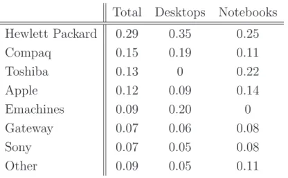
NPD Techworld via automatic feeds from their participating outlets on a weekly basis.11 The data cover the course of 90 months, November 2001 to April 2009, and consist of sales occurring at outlet stores. Thus, manufacturers such as Dell that primarily sell directly to the consumer are not included. Each observation consists of a model identification number, specifications for that model, the total units sold, and revenue. From units sold and revenue we calculate a unit price of each PC sold. Table 1 displays the share of units sold in the data for the entire sample and as well as for the notebook and desktop subsamples. Hewlett Packard and Compaq make up the bulk of computers sold in the

data, at 29 and 15 percent, respectively.12

In the TUP survey data, we have access to four annual surveys that were conducted from 2001 to 2004. TUP is a detailed two-stage survey of households’ use of information technology and consumer electronics products and services at home and in the workplace. The first stage is a screener, which asks for the characteristics of each head of household (such as income, education level, marital status, and presence of children). The second stage consists of the technology survey, which asks a multitude of questions ranging from

brand, to year of purchase, to where the computer is used. 13

2.1

NPD Data

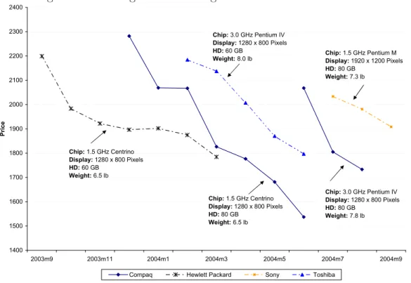
We use the NPD data to document the differences between pricing, sales, and tech-nology adoption by Apple and PC manufacturers. Figure 1 highlights these major differ-ences, where each point in the figure represents the unit price for a particular computer model in the sample of 15-inch notebook computers. The price time series for a given

computer model is created by linking the model’s prices over its life on the market.14 _The

11_{The weekly data are organized into monthly data using the Atkins Month Definition, where the}

first, second and third months of the quarter include four, four and five weeks, respectively.

12_{While Hewlett Packard and Compaq merged in 2003 we chose to keep the firms separate in our}

analysis.

13_{All observations are reported on the user’s “primary computer.” An observation in this data consists}

of household demographics and computer specifications including the price paid. We isolate observations where PC is used at home, and we drop observations where the specification of PC is not reported.

14_{For ease of view, prices after the units CDF reached 90 percent for each model were omitted. We also}

three “PC” manufacturers (Hewlett Packard, Sony, and Toshiba) have short product cy-cles, frequent staggered entry, and declining prices over the life of the good. In contrast, Apple, has long product cycles, less frequent and more uniform entry, and flatter price contours. Below, we show that these these patterns are consistent with the personal computer industry as a whole.

2.1.1 Product Cycle Length

Focusing first on the length of the product cycle, we construct CDFs by manufacturer, as well as for the sample of all PCs (i.e. all manufacturers other than Apple) in Figure

2.15 _{On average, PC manufacturers sell well over half (64 percent) of their units by the}

second month on the market, and by the third month they have sold close to 90 percent of their units. Apple, however, keeps its computers on the market about twice as long as the other PC manufacturers. By the third month, when the PC manufacturers have sold almost all of their units, Apple has sold only 38 percent of its total units. In fact, Apple does not reach the 90 percent marker until its product has been on the market for at least seven months.

The fact that Apple holds its computers on the market for a longer period of time does not necessarily mean that it introduces new computers less frequently. For instance, Apple could very well be staggering the introduction of its new computers in such a way that it is releasing a new computer every period. Our data, however, show that this is not the case. Table 2 reports the fraction of months in the sample where no new computer was introduced. This is in effect measuring the fraction of months in which the manufacturer’s entire product space is composed of computers that are at least one month old. Of the seven manufacturers, Apple has the largest proportion of months where no new models are introduced (28 percent); by contrast, Hewlett Packard had only one month in the sample with no introduction of a new model.

Table 2 also depicts the maximum amount of time the manufacturer goes without

15 thousand for Sony and Toshiba, and 4 thousand for Apple.

15_{We measure the CDF by running a regression of monthly unit sales on “months on market” dummies}

creating predicted values of the number of units sold given months on the market. Because computers do not necessarily enter the market at the beginning of the month, the first month of data will include less than 31 days worth of units sold. See Appendix A for details.

introducing a new model. These numbers also show that Apple is relatively slow to introduce new computers. For instance, Apple underwent a period of nine months in which it did not introduce a new desktop computer, and a period of six months without introducing a new notebook computer—by far the longest periods in the sample.

Thus far we have been discussing the introduction of new computers into the market. For computer firms, we argue that new computers frequently incorporate a new upstream innovation. Consequently, the rate at which a computer manufacturer adopts new com-puters is the rate at which the manufacturer is adopting new technologies and embedding them into its products. Our reasoning for equating product entry with technology adop-tion is based on the producadop-tion technology for computers. Computers have many internal components which are produced by a diverse array of distinct upstream firms. Upstream firms undertake R&D in an attempt to increase the quality of these components that they sell to the downstream computer manufacturers. Computer manufacturers, con-sequently, have ample opportunity to adopt new technologies when introducing a new computer to the retail market. For instance, one month Intel may introduce a new CPU, while the following month Samsung may introduce a new DRAM chip. The large number of components, as well as the complexity of the quality of the components, make it a nontrivial task to monitor and measure their adoption by computer manufacturers. In-stead, because we focus on the industry as a whole, we make the assumption that newer components are more innovative, and thus an introduction of a new computer model (i.e. SKU) is synonymous with new technology adoption. While this assumption could be flawed if, for instance, CPU manufacturers are frequently crimping their products, we believe that it is a realistic assumption in the sense that newer computers generally embody more innovative, higher quality components.

Supporting evidence that Apple adopts and introduces new innovations at a slower pace relative to PC manufactures can be found by looking at CPUs, arguably the most important component of the computer. To gauge how frequently manufacturers adopt new CPUs, we plot the age of the newest Intel CPU by month for the post-PowerPC

period for Hewlett Packard, Toshiba, and Apple notebook computers in Figure 5.16 _Two

16_{The age of the CPU was calculated by subtracting the current time period from the period in which}

the chip first appears in our sample. Apple switched from Motorola/IBM powerPC chips to Intel chips in June of 2006. We depict notebook computers in the figure because Apple’s desktops use Intel Xeon

features of this figure are striking. First, Toshiba and Hewlett Packard are twice as often the first to adopt a new CPU (12 and 14 months out of 35, respectively) as Apple (7 out of 35 months). Second, Hewlett Packard and Toshiba rarely keep a CPU beyond its three month anniversary, while on three occasions, Apple’s newest CPU available was seven months old. Table 3 shows CPU adoption statistics for the entire sample of notebook computers and shows that, on average, Apple offers the oldest CPU for this sample period. The CPU evidence, then, shows how Apple introduces innovations into their computers with a lag compared to PC manufacturers. Hence, the more rapid rate of product entry of PCs allows PC manufacturers to more quickly incorporate the latest innovation relative to Apple.

2.1.2 Pricing Patterns

Alongside the shorter product cycle and more rapid rate of product entry, Figure 1 highlights stark differences in the pricing dynamics between PC manufacturers and Apple. Generally speaking, Apple maintains a flat price profile over a computer’s product cycle. In contrast, PC manufacturers introduce their products at a high price and then lower that price over the product cycle. We measure the rate at which prices fall over the life of the computer by estimating a fixed-effects regression of the logarithm of price on “months on market” variables for each brand in the sample. Figure 4 depicts the results of these regressions and highlights the extent to which each brand reduces the price of the computer over the life cycle. Depicted are the estimated coefficients for the first six months of the life of the good. The omitted dummy variable is the first month of entry indicating that the subsequent coefficients represent the percentage change between the

given month and the first month.17

It is clear from Figure 4 that Apple’s prices fall relatively slowly and less extensively than do the prices of the PC manufacturers. For instance, Hewlett Packard and Toshiba’s prices fall by 9 and 12 percent, respectively, between the first and fourth months. On

processors, which cannot be differentiated by processor name in the data.

17_{We describe the fixed-effect regression analysis in Appendix A, where we provide a table of estimates}

and their standard errors for months 2 through 12 of the product cycle. Because many of the price declines in the latter part of a product’s life cycle are due to stock-out sales, we also report estimates where we omitted observations beyond the 90th percentile of the units CDF function.

average, a PC falls in price 6 percent by the third month, 10 percent by the fourth month, and 18 percent by the fifth month. In contrast, Apple’s prices show negligible price declines over these same time horizons: 0.4 percent, 0.9 percent, and 1.7 percent, respectively.

It is important to discuss how these pricing patterns fit into the predictions of theories on durable goods pricing. There have been many theories that have been developed by researchers to describe the falling pricing patterns for durable goods. Process innovation and intertemporal price discrimination are two such explanations which have received a large amount of attention. At most, declining input costs due to process innovation can explain a small fraction of the observed price declines for PCs. The average price decline of 10 percent for PC computers over 4 months translates into a 30 percent price decline at an annual rate. Prices for screens, batteries, and other components of PCs do not decline at such a rapid rate. Furthermore, Apple uses many of the same intermediate inputs used by PCs, yet its prices only negligible decline over time. Consequently, we rule out process innovation as a main driver behind falling PC prices.

Intertemporal price discrimination, whereby the firm charges a high price early in the product cycle to those with highest willingness-to-pay, seems like a plausible candidate at first glance. Stokey’s (1979) ground-breaking analysis, however, showed that such price discrimination is profit maximizing only under very strict assumptions. First off, the firm needs a considerable amount of market power, otherwise competitive forces will determine the price. Second, consumers’ reservation prices must be correlated with their time preferences, otherwise high willingness-to-pay consumers would prefer to wait for the price to fall. Finally, the firm must have the ability to commit to future prices or

production to avoid the time inconsistency dilemma posed by Coase.18 _{Thus, if the price}

falls in the PC market are due to intertemporal price discrimination, than it must be the case that for some particular reason Stokey’s conditions are met in the PC market but not the Apple market. We have no reason to believe that willingness to pay is more correlated with time preference for consumers in the PC market than for consumers in the Apple market. Furthermore, market power should be positively correlated with a firms

18_{Bulow (1984) shows that a firm will “oversell,” use an inefficient production technology, or produce}

ability to commit to a price or production schedule. Unless Apple hasless market power than the PC manufacturers, intertemporal price discrimination seems like an unlikely candidate for the declining pricing patterns.

Unlike declining input costs and price discrimination, competition seems to be a plau-sible force behind declining PC prices over the product cycle. It is conceivable that the frequent adoption of higher quality PCs can drive down the prices of PCs currently on the market. Indeed, there are interesting dynamics between prices and product entry among PC manufacturers. In particular, PC manufacturers often leapfrog one another with the introduction of new, higher quality computers. To display this feature in the data, in Figure 5 we isolate 512 MB RAM 15-inch notebooks where the entering PC happened to be the highest price in this product line. This exercise attempts to isolate the computer models with both the newest and highest quality technology under the assumption that the computer with the highest quality is also the highest priced. Supporting our claim that newer products are of higher quality, we also report four computer characteristics highlighting in which dimension the newly introduced computer is of higher quality rel-ative to the incumbent computers. The manufacturer with the highest quality 512 MB RAM 15-inch notebook rotates between Hewlett Packard, Compaq, Toshiba, and Sony. Introductory prices of these computers are quite high, around $2,100, but then quickly fall to $1,800. In line with the story that competition drives the observed price declines, the introduction of the new model seems to put downward pressure on the preceding model as is the case with the introduction of Sony’s product.

Looking ahead, in section 3 we develop a formal industry model of the personal computer industry. The model generates price declines over the product cycle through competitive effects, much like we observe for PC manufacturers. These price declines, along with decreasing sales, subsequently increase the incentives for adopting a new technology and ultimately drive the product off the market.

2.2

TUP Survey Data

In addition to the firm side, there are important features of the personal computer industry on the consumer side. In this section we highlight some facts about the under-lying distribution of consumers purchasing PCs using the TUP survey data. We focus

on consumer income as it is typically closely linked to reservation price, and therefore product choice, in most econometric studies and economic models. The survey data re-veal that both the levels and distributions of income differ across brands in the industry. Furthermore, we also document that income is correlated with the price paid, holding fixed the characteristics of the computer.

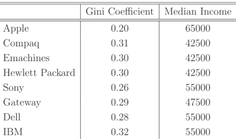
There are large differences in the income distribution of Apple consumers and PC consumers. Table 4 highlights these differences by showing the median income and dis-persion of income (represented by the gini-coefficient) for each brand in the TUP survey

data.19 _{The survey data show that consumers of Apple have narrow income dispersion}

(0.195 gini coefficient) around a relatively high median income level ($65,000).20 _In

con-trast, the PC brands have consumers with much wider income dispersions around lower median levels.

Using the same TUP survey data that we use in this study, Aizcorbe and Shapiro (2010) find that higher income consumers pay a higher price for the same computer than do lower income consumers. Specifically, a fixed effects regression is run–holding fixed the attributes of the computer purchased–of income and other demographic variables on the logarithm of price. The study finds that the coefficient on income is .09 indicating that a 9 percent fall in a consumer’s income is correlated with a 0.9 percent fall in the price paid for a given computer. Combining these results with the price declines observed for PCs, shows that high-income consumers are presumably purchasing early in the model’s

life cycle.21 _{Naturally, because Apple’s prices remain flat over the computer’s product}

cycle, there is no correlation between price and income.

It is not obvious why the income distributions between the two markets differ. It could

19_{The gini-coefficient represents twice the expected absolute difference between two individuals’}

in-come drawn randomly from the population. Thus, the larger the gini-coefficient the wider the degree of dispersion.

20_{We note that these dispersion statistics are somewhat prone to measurement error due to the}

placement of income levels into bins. Each income level represents the midpoint of the bin, expect for the last bin which is $150,000 and greater. Therefore, if a large proportion of Apple’s consumers have incomes much greater than $150,000, the gini on Apple could realistically be somewhat larger than what we measure.

21_{Interactions between brand and income also verify that the correlation between income and price}

very well be that Apple targets high income consumers, while PC manufacturers target an array of consumer types. The model we develop in the next section, however, compels us to believe that this is not the case. Specifically, the model posits that competitive forces lower prices sequentially over the product cycle, drawing in lower income consumers to purchase the product. Thus, we show that the degree of consumer heterogeneity in the market can be endogenously determined by market structure.

3

Model of the The Competitive Industry

In this section, we consider the competitive industry where firms compete with one another over products that are perfect horizontal substitutes (e.g. the same product line, such as 15-inch notebook computers running on the IBM platform) but imperfect vertical

substitutes (e.g. differing degrees of quality, such as CPU clock speed).22 _{As in Shaked}

and Sutton (SS), single product firms compete with one another in price while taking into account the distribution of consumer taste over quality. Unlike SS, we consider a dynamic game where firms also choose when to update the quality of their products. In steady state, the model produces predictions of the price and sales path of a computer over its life cycle.

After introducing the model, we measure the model’s fit with the data by comparing the price and sales paths generated by the model with that actually seen in data. Our results indicate that the model does a nice job of explaining the data for IBM platform PCs. We then discuss the model’s implications about the effects of product entry on pricing and sales dynamics.

3.1

The Competitive Model

We model the competitive computer industry using an infinite-period vintage-capital

model. Computers are differentiated by their vintage ν, where ν equals the date at

which a vintage is the frontier technology; at time t, the frontier technology is ν =t. In

essence, vintage is a proxy for quality where newer vintages are of higher quality. There

22_{In the following section, we look at the monopolistic industry where the firm is the sole provider of}

is an outside option, which provides utility,ˇut, to a consumer in periodt. Over time, the utility of the outside option increases.

We set the number of firms in the market to beN, and so consider our analysis to be

in the short run. Further, we simplify the problem by assuming that each firm produces at most one computer, and so ignore any joint maximization problem of a multi-product line firm. Thus, we can think of the model as characterizing firms competing over a specific product line, such as the 15-inch 512MB laptop computers depicted in Figure 5.

3.1.1 Demand

Each period, a mass of consumers enter the market. Consumers either buy one com-puter, or choose the outside option. In both cases, consumers leave the market at the end of the period, so there is no accumulation of consumers across periods. Consumers

are differentiated by their budgets for computers and related products, denoted y.

Con-sumers gain utility from purchasing a computer and from using the remainder of their

income to purchase some alternative computer-related good such as software. Let pνt

denote the time tprice of vintageν. We normalize the price of the outside good to zero.

Following SS we assume the consumer’s utility from purchasing the computer of

vintage ν is

U(y, ν; ¯pt) =uν ·(y−pνt) (1)

where ¯pt is a vector of prices and uν represents the quality of a computer of vintage ν.

We make the natural assumption that newer vintages are preferred to older ones, and so

ut > ut−1 ∀t. The utility from the outside good is ˇ

ut·y. (2)

Given prices, the consumer’s utility-maximization problem is: max ½ max ν∈ν¯t U(y, ν; ¯pt), uˇt·y ¾ , (3)

where ¯νt denotes the set of available computers in period t. The resulting demand

function is straightforward.23 _{We order the vintages by their utility levels and consider}

23_{This is the demand system of Prescott and Visscher (1977), which has been well-studied in the}

the neighboring vintagesνkandνj whereuk < uj. Given that the lower quality computer has a lower price,pνk < pνj, there is a marginal consumer with income ˆy, who is indifferent between them:

uνj ·(ˆy−pνj,t) = uνk ·(ˆy−pνk,t). (4)

All consumers with income less than ˆy prefer νk overνj and all those with income more

than ˆy prefer νj over νk; denote this marginal consumer yνk,νj. Repeating this exercise

across all pairs of neighboring vintages, we can define a set of marginal consumers from which demand for each computer vintage can be computed. Consumers between the marginal consumers (yνl,νk, yνk,νj) will purchase vintage νk. The demand for νk is then simply Qνk = Z _y νk,νj y_νl,νk h(x)dx,

where h is the distribution of consumer’s income. Given the ordering of vintages, ν1 is

the best available product. Its demand is given by

Qν1 =

Z _∞

yν₂,ν₁

h(x)dx.

Similarly, let νN be the lowest quality product. It competes directly with the outside

option, and its demand is given by

QνN =

Z _y

νN ,νN−1

y_u,νNˇ

h(x)dx,

where yˇu,νN solves

uνN ·(y−pν,t) = ˇut·y.

3.1.2 Supply

A firm makes two decisions each period. At the beginning of the period, it sets a price for its computer. At the end of each period, the firm decides whether or not to adopt a new technology (i.e. update its product). If the firm adopts, its computer embodies the

latest technology in the next period. Letting i= 1,2, . . . , N denote a firm, we label the

decision to adopt the latest technology as dit ∈ {0,1}, where d = 1 signifies adoption.

We assume firms have a constant marginal cost c≥0 and no capacity constraints. The

state variables are st = (ν1, ν2, . . . , νN,uˇt), which consist of all firms’ products and the

outside option. Let δ = 0.99 denote the discount rate, then firm i’s profit-maximizing

problem is: Vi(st) = max p_νit,dit ½ (pνit−c)Qνit(pνit, pν−it;st)+ δhdit(Es0[V_i(s0)]−φ) + (1−d_it)E_s00[V_i(s00)] i¾ , (5)

where pν−it denotes all other firms’ prices in time t, given st. Qνit is the demand for

product νi at time t, given prices and the outside option. If the firm decides to adopt,

next period it pays the sunk costφand acquires the latest vintage, ν0 _{=t+1. Otherwise,}

the firm continues to sell its current computer. Expectations are taken over the evolution

of st, which depends both on the firm’s own updating decision, as well as all other firms’

decisions.

While the firm’s price-setting decision is static, its adopting decision is dynamic. Because consumers value quality, updating to the latest technology generates higher

revenues for the firm, holding all else constant. But, the firm pays a sunk cost φ to

acquire the latest technology. Hence, the firm balances the gains to adopting in the current period against the option value of continuing to sell its computer and upgrading in the future.

Rather than physically depreciate, a computer faces two sources of obsolescence over time. First, the outside product is assumed to improve over time; therefore, in each

successive period, a computer with vintage ν maintains its utility value to consumers

while the outside option becomes more attractive. This general obsolescence places

downward pressure on prices of existing computers. Second, with each successive period other firms may update their computers. Newer vintages, embodying better technologies,

directly compete with a vintage ν and drive down its price. We label this second source

of obsolescence market-specific obsolescence.

periods. After some point, the demand for a product when priced at marginal cost will equal zero and effectively the computer will have exited the market. Of course, a firm may decide to adopt a new model before demand reaches zero. The life cycle of a computer, then, starts with its introduction into the market and ends when either the firm adopts or there is no longer demand for the computer at a price greater than marginal cost.

3.1.3 Equilibrium concept

We use a Markov perfect equilibrium concept. The strategy space includes price and adoption, and firms’ actions are functions of the current vintages of computers offered

along with the utility value of the outside option, st. Firms maximize the expected

dis-counted value of profits, conditional on their expectations of the evolution of the state variables and competing firms’ strategies. Equilibrium occurs when all firms’ expecta-tions are consistent with the evolution of both the outside good’s utility as well as all the optimal pricing and adopting policies of their competitors.

To fit the model to the data, we consider a stationary Markov perfect equilibrium. The model will be stationary in the sense that prices and sales of a computer over its life cycle will be independent of time. To obtain a stationary equilibrium, we make an additional assumption: the ratio of the utility associated with a computer embodying the frontier technology over the utility provided by the outside good remains constant over time. Formally,

ˇ

ut νt

=ζ ∀t (6)

A stationary equilibrium occurs when firms use the following strategy: the firm with the lowest-quality computer adopts and all other firms do not upgrade. For pricing, each firm’s strategy is to use its best-response function to choose price. From SS, we know that given a set of products, there exists a Nash equilibrium in prices.

3.2

Empirical Fit

Given a vector of parameters, we compare the model’s predictions of prices and sales of a computer over its product cycle to those observed in the data. We parameterize the

competitive model to match the sales and prices of the average PC.

3.2.1 Description of Parameters

The parameters of the model can be categorized into three groups. The first set of parameters determine the quality level of computers relative to each other and the outside good; the second set characterize the consumers’ income distribution parameters, and the third set detail the cost structure of the firm. We use three parameters to characterize

computers’ quality levels: (i) The level of the highest quality product, ν1, which we

normalize to 10, (ii) the monthly growth rate of the frontier technology, γ, which, based

on Moore’s law, we set to 2.9 percent, and (iii) ratio of the outside good’s to highest

possible quality product’s utility, ζ, which we set to 0.01.24

The substitutability of products across vintages is determined by γ. Raising γ

en-larges the difference in utility associated with the newer vintage relative to the older vintage increases, decreasing substitutability across vintages. The attractiveness of the

outside good relative to products is determined by ζ. As ζ approaches one from below,

the outside good becomes more attractive relative to the frontier technology.

We assume consumers’ budgets for computers and related products is drawn from

the Uniform distribution over the interval [a, b]. We normalize a to be one, but leave b

free. The upper bound of income plays a large role in determining the total number of

products the market is able to support (see SS). The density of consumers over [a, b] is

given by κ >0.

Finally, we assume a simple cost structure for the firm. The firm pays a sunk cost,

φ >0 to enter the market. Upon entry, the firm’s production technology has a constant

marginal cost, mc >0. The model provides an upper bound to the value ofφ, in thatφ

must be less than a product’s present discount value of lifetime profits.

This leaves three free parameters in our model, θ ={b, κ, mc}. Given these

param-eters and the equilibrium adoption condition, the model yields predictions about price and sales for a product over its life cycle in the steady state. As discussed in Section 2, it is difficult to measure the rate at which upstream firms are introducing new components

24_{While we use Moore’s law as an indicator for the rapid increase in computer quality overtime, our}

into the market for any specific product market. For example, an innovation for a spe-cific monitor technology may only be relevant for small laptop computers while a certain innovation in CPU technology may only be relevant for large desktop computers. Thus, there may be different available technologies depending on the product line, and these innovations may arrive at different rates. As such, we consider four different patterns at which upstream firms introduce new components: every period, every second period, every third period, and every fourth period. Firms’ adopting strategies for these different innovation patterns remain the same: only the firm with the lowest quality computer adopts the new technology. The opportunity of adopting, however, arrives every second, third, or fourth period, while the outside good is growing at a constant rate every

pe-riod. Given θ, we solve the model for each innovation pattern and record the price and

sales path of a product over its life cycle. We then take a weighted average of the four

price and sales paths, using the weights ω={ω1, ω2, ω3, ω4}. Interpreting the weights as

probabilities, this average is the expected price and sales paths of a computer over its life cycle.

3.2.2 Results

To compare the model to the data, we compute price declines and the sales CDF from the expected price and sales paths. In the data, we estimate these average price declines and sales CDF using fixed-effect regressions (see Section 2.1). To most closely

align the model with the data, we find the pair {θ, ω} that minimizes a least-distance

criterion.25

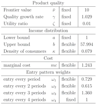
Table (5) displays the parameters that best match the model to the data. There is a wide distribution in budgets for computers and related products. Those consumers with the largest budgets are willing to spend more than 58 times the amount of those consumers with the smallest budgets. Further, marginal cost is low enough that almost all consumers purchase a computer. The estimated weights across the four entry patterns place the largest weight on entry every 3 periods, and the least weight on entry every 2 periods.

As displayed in Table (6), the model fits the data well along both the price and sales

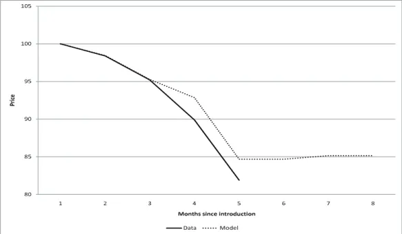
dimensions. Turning to sales first, the model matches the large burst of sales in the first month a computer is introduced. As shown more clearly in Figure (7), the model captures the fact that computer sales decline over the product cycle. In addition, the model predicts that more than 95 percent of a computer’s sales occur by month 5 of the product cycle, closely matching what we observe in the data. Unlike the data, the model does predict a trickle of sales over months 6 through 12 of the product cycle which we argue are economically insignificant.

The model does an excellent job of matching the price declines seen in the data (see Table (6)). To provide a visual display of the model’s fit to the data, in Figure (6)) we plot the price levels for the model and data fixing the price in period one to 100 for both cases. For the tiny amount of sales in months 6 through 12, the model predicts a flat price profile. This reflects the fact that computers sold many months after their introduction are the lowest-quality computer available. Consequently, prices are only slightly above marginal cost and cannot fall. As mentioned above, while we report prices for months 6 through 12, we attach little importance to them.

These results demonstrate that the competitive model is able to closely match the price and sales patterns observed in the IBM platform PC data. In a goodness-of-fit measure, we compare the model’s predictions on the timing of a household’s purchase decision, conditional on its budget. As described in Section 2, the TUP survey data imply that households with higher incomes purchase computers earlier in the product cycle. Aizcorbe and Shapiro (2009) find that a 0.9 percent fall in price is correlated with a 10 percent fall in income. Under the assumption that a household’s budget for computers and related products is positively correlated with its income, the model also predicts that higher income households purchase computers earlier in the product cycle. In Table (7) we compute the average budget of consumers for a computer over the product cycle for each entry pattern. The average budget of consumers who purchase the highest-quality computer is 90 percent larger than those who purchase the second highest quality computer. While the model seems to over-predict the fall in consumers’ budgets over the product cycle, we believe this is mainly due to our assumption that

consumers’ budgets are uniformly distributed.26 _{A more flexible distribution would likely}

preserve the model’s fit to the price and sales moments, while generating a more gentle decline in consumers’ budgets over the product cycle.

Finally, the model implies reasonable markups. When a computer is the newest vintage available, manufacturers charge an average markup of 25 percent. Once a newer vintage enters the market, however, this markup plummets to about 1 percent.

3.3

Analysis

To examine how technological adoption impacts prices and sales, we compare the model’s predictions across the four upstream-firm innovation patterns. In Figures 8 and 9 we plot prices and sales over the product cycle for each case, alongside the average

across all cases.27 _{There are three active firms across all four cases. In steady-state, this}

implies a product cycle of 3,6, 9 and 12 months respectively.

Turning first to prices, we see that the introduction price is rising as opportunities for adoption occur less frequently. This pattern reflects the level of substitutability across vintages. When upstream innovation is slower to arrive, adoption occurs less frequently and there are larger differences in quality among computers on the market, decreasing their substitutability. The lesser degree of competition therefore allows the manufacturer to charge a higher initial price for its new product. Over a computer’s life cycle, there are two basic price levels. When the computer is the highest quality product available, the firm charges a high price and has a significant markup. Once a computer is no longer the highest quality product, the firm charges a low price which is slightly above marginal cost. The dramatic fall in price as a computer changes from highest quality to second highest quality is a result of the fierce price competition among manufacturers.

Similar to prices, there are two basic sales levels over a computer’s life cycle. A manufacturer commandeers over 90 percent of the market its computer is the newest vintage available. When the computer is no longer the newest available vintage, however, sales dramatically fall. The large decline in sales is especially striking because prices are

27_{The “Average” line in Figures 8 and 9 is the average across all four cases, using our estimated}

weights. These averages are the expected price and sales paths over the product cycle. Using this expected price and sales figures, we compute the price declines and sales cdf figures used to fit the model to the data.

also dropping. Therefore, the firm with the highest-quality computer is able dominate the market, achieving a high level of sales as well as a higher price. Competition from a newly adopted, higher quality products subsequently erodes any firm’s market dominance.

Because the newest vintage computer dominates the market, the reward to a man-ufacturer for updating its computer with the latest technology is substantial. In the language of the innovation literature, there are high post-innovation rents because the highest quality computer captures over 90 percent of the market while charging a high price. Furthermore, there are low pre-innovation rents because once a computer is no

longer the highest quality, its sales and price are low.28 _{The main driver behind a firm’s}

updating decision is the size of the difference between post- and pre-innovation rents (Ar-row 1962 and Aghion et. al 2001, 2005). In the competitive environment of our model, the difference between the post- and pre-innovation rents are substantial. This difference in post- and pre-innovation rents is driven by competitive effects, or market-specific ob-solescence. In contrast, the role of general obsolescence, captured by the growth rate of the outside good, plays at most a small role in the model’s predictions of prices and sales. This is significant because, in a market structure without competition (i.e. monopoly), the only force driving the firm to update its computer is general obsolescence. As de-tailed in the following section, without competition a manufacturer faces much less of an incentive to adopt a new technology.

4

The Monopolistic Industry

We now consider the monopolist’s problem, with the goal of determining how much market structure alone explains the differences in sales, prices, and adopting between PC and Apple manufacturers. The monopolist’s problem is equivalent to the competitive case outlined earlier, except that there is only one firm. The difference is that the competitive firm faces technology adoption by other firms, while the monopolist need only worry about general obsolescence stemming from growth in quality of the outside

28_{This is a different approach to the original Schumpeter idea which was looking at the incentives for}

outsiderfirms—firms just entering the market—where only the level of the post-innovation is important, since the pre-innovation rent is always zero.

good. Consistent with the competitive case, we assume that the monopolist sells only one product at a time.

4.1

The Monopolist’s Problem

The timing of the monopolist problem is the same as the competitive case. At the beginning of the period, the monopolist chooses price. At the end of the period the monopolist chooses whether or not to update its product. The state space of the

monopolist in periodt is its existing productνsand outside option, ˇut. The monopolist’s

problem is V(νs,uˇt) = max pνs,dt ½ (pνs −c)Qt(pνs;νs,uˇt)+ δ h dt([V(νt+1,uˇt+1)]−φ) + (1−dt)[V(νs,uˇt+1)] i¾ . (7) Like the competitive firm, the monopolist’s adoption problem balances the gains from introducing a computer in the current period, against waiting a period (or more) to do so. Bringing out a new vintage increases profits because consumers are willing to pay more for a superior product. However, the introduction of a new computer entails paying

a sunk cost, φ.

4.2

Out-of-Sample Prediction

To determine how much market structure drives the different pricing, sales, and adop-tion patterns across PC and Apples, we perform an out-of-sample predicadop-tion exercise.

Using the sameθas in the competitive case, we solve for the monopolist’s optimal pricing

and updating strategy. Formally, we keep preferences and technology fixed, but change the market structure by reducing the number of firms to one. We then simulate the model and compare its predictions of prices and sales over the computer’s life cycle to what we observe in the data. As detailed below, the model’s out-of-sample prediction is closely aligned with the Apple computer data. Hence, the model predicts that market structure is the main force behind the different pricing and sales for PC and Apple com-puters. Furthermore, the model predicts that competition drives PC manufacturers to

update their computers more frequently and adopt the latest innovations more rapidly relative to their Apple counterpart.

In taking the monopolist’s problem to the data, a key parameter is the sunk cost of

updating, φ. Indeed, the frequency with which the monopolist updates its computer is

directly linked to φ. Because the outside option grows over time, the price charged and

per-period profits earned by the monopolist decline with the vintage of the computer (see Figure 12); however, the monopolist does not update its computer every period, because of the sunk cost of replacement. Intuitively, the larger the sunk cost, the less frequently the monopolist updates its computer. In Figure 13, we plot the optimal replacement cycle length against the sunk cost of replacement. With a sunk cost of replacement of 0.05, the monopolist chooses to update its computer every 2 periods. If the sunk cost of replacement is 2.0, the monopolist chooses to update its computer every 13 periods.

The competitive case only provides an upper bound ofφ.29 _{Given this constraint, we}

choose a sunk cost of entry such that the model’s prediction on the monopolist’s timing of replacement matches the data. We infer that Apple’s computers are sold for 8 months

on average. To match this replacement cycle, we set φ to be 0.7, or 18 percent of the

expected discounted profits of a firm in the competitive market. Thus, the parameter value chosen for the cost of adoption is consistent with the results from the competitive case presented earlier.

Givenθandφ, the model predicts a flat price profile over the product cycle (see Table

8), a close match to the prices of Apple computers seen in the data. Specifically, Apple’s price declines are negligible for three-quarters of the product cycle, before being heavily discounted. The data show Apple’s average prices fall so dramatically after month six is because of occasional product replacement. When Apple introduces a new vintage, the

stock of existing computers is heavily discounted.30 _{Since our model does not account for}

29_{Using a discount rate equal to 0.99, we use our model’s results to compute a product’s lifetime}

profits for each entry pattern in the competitive case. We then use the estimated weights to obtain expected lifetime products from entry, ˆπ. To ensure that manufacturers are willing to introduce a new product, it must be that the sunk cost of entry is less than expected profits, orφ <πˆ.

30_{These pricing dynamics can be seen in Appendix C, which depicts the price contours of four of}

Apple’s notebook product lines: 12-inch PowerBooks, 14-inch iBooks, 15-inch PowerBooks, and 17-inch PowerBooks. Prior to replacement the average price fall (where we average over number of periods) of

such stock-out sales, it is unable to match the sharp falls seen later in the product’s life.31 In Figure (10) we plot the price levels predicted by the model against those observed in the data for a typical computer over the product cycle.

The model closely matches the steady flow of sales throughout the product cycle. As seen in Table (8), the sales CDF generated by the model closely follows what we observe in the data, although the model does predict a lower level of sales at the beginning of the product cycle. Figure 11 illustrates this disparity, as the sales PDF for the model and data are plotted next to one another. In the data, we see a decline in sales over the product cycle, but we do not see a corresponding decline in the model. The decline in monthly sales volume, however, is actually quite small. In its first month, sales are almost 17 percent of total sales over the product cycle. In the sixth month of the product cycle, sales are still 13 percent of total sales, which amounts to only a small decline. Admittedly, in the last two months of the product cycle, sales decline in the data but not in our model. As mentioned above, however, we believe this behavior reflects fire-sales by Apple because of the introduction of a replacement computer; we do not account for this behavior in our vintage capital model.

Overall, with only a change in market structure, our parsimonious model is able to capture the flat price profile of Apple computers along with the steady flow of sales throughout the product cycle. Finally, the 8 month long product cycle for the typical Apple computer is captured using a reasonable sunk cost of updating, an amount equal to 18 percent of the expected discounted profits a firm in the competitive market receives. Further supporting the fit of the model to the data, the model’s predictions on prices and consumers’ budgets roughly accords with the data. In stark contrast to the competitive case, in the monopoly setting the average budget of consumers purchasing a computer at different vintages remains roughly constant (see Table 9). In addition, the average budget of a household which purchases a computer in the monopolistic setting is higher than in

these four product lines is 0.1, 0.02, 0.7, and 0.4 percent, respectively. However, the average price fall in the period directly after replacement(where we average over number of models) are 5.4, 6.5, 9.6, and 5.2 percent, respectively.

31_{Because the arrival of a replacement product can only be found by visually looking at distinct}

product lines and using detailed knowledge of the industry, we found no systematic way to correct for stock-out sales throughout the entire dataset.

the competitive setting. Under the assumption that consumers’ budgets for computer and related products are positively correlated with household income, our model matches the income data from TUP survey data: the distribution of consumers’ income in the monopoly setting has a higher mean and a smaller variance relative to the distribution of consumers’ income in the competitive setting.

5

Welfare Analysis

We assess the welfare effects associated with technological adoption by examining producer and consumer surplus under the four upstream-firm innovation patterns we analyzed in the competitive market. Recall that a slower rate of upstream-firm innovation translates into slower arrival of opportunities for technology adoption. We then look at consumer surplus in the monopolistic market. A priori, welfare can either increase or decrease with faster rates of adoption. Consumers are better off with more frequent adoption because of quicker availability of higher quality products and the more rapid

fall in prices.32 _{Firms, however, generate lower profits with more frequent adoption rates}

since they pay larger total sunk costs and charge lower markups.

To allow for comparison over different product cycles, we compute the firm’s dis-counted profits over 72 periods. We decompose profits into producer surplus and the sunk costs of adoption, where producer surplus is the firm’s markup times sales. In level terms, producer surplus rapidly increases and sunk costs fall as entry occurs less frequently (see Table 10). Indeed, producer surplus is four times greater when entry occurs every 4 periods relative to entry every period.

We measure consumer surplus as the difference between a consumer’s willingness-to-pay and the price the consumer actually paid for a computer in equilibrium. To compute willingness-to-pay, we find the price at which a consumer is indifferent between the computer he originally purchased and the outside option. Formally, for a consumer

32_{We note that our model ignores network effects. Ellison and Fudenberg (2000) show that as network}

externalities become more important, it becomes socially optimal for the firm to sometimes withhold innovations.

with budget y who purchased a computer of vintage ν, we solve for the ˆp such that

uν(y−pˆ) = ˇuy. (8)

Rearranging terms, we get ˆp= (1− uˇ

uν)y. The difference between ˆpand the equilibrium

price represents an individual consumer’s surplus. We integrate over all consumers who purchased a computer to compute total welfare. To allow for a proper comparison with producer surplus, we compute consumer welfare, properly discounted, over 72 periods.

Table 10 indicates by how much consumer surplus, producer surplus and sunk costs change with different rates of adoption. We find consumer surplus falls with slower rates of entry. While this decline is tiny in percentage terms, consumer surplus is so large that these small percentage changes more than offset the increase in firms’ profits. Consequently, total welfare falls as entry rates slow down.

Comparing welfare in the competitive and monopoly cases, we find that total welfare under a monopolist is roughly three-fourths of the level in the competitive case. As shown in Table 10, the monopolist is able to capture two-thirds of total welfare. Consumer welfare under a monopoly is much smaller compared to the competitive case, because of both higher prices and a much smaller set of consumers purchasing a computer.

As our model abstracts from some important features of both the PC and Apple markets, our welfare results should be taken with some caution. Among other things, we do not account for the difference in quality between operating systems across the two retail markets, nor do we take into account the network effects related to the depth of software offered. Bearing this in mind, our results indicate that total welfare is increasing with faster rates of adoption. This stems from the fact that consumers receive a large benefit from rapidly declining prices and availability of higher quality products from frequent adoption. This large benefit supersedes the fall in producer surplus that rapid adoption entails.

6

Concluding Remarks

Our key contribution is assessing the role that market structure plays in the frequency of new technology adoption. Our strategy was to parameterize a model of vertically

differentiated firms to fit “PC” prices and sales, and then perform an out-of-sample prediction where we remove the effects of competition from the model. The out-of-sample exercise produced a time path of prices and sales that closely match that of Apple, a computer manufacturer with a large degree of market power due to its horizontal differentiation in operating system. Importantly, the model demonstrated that relative to the competitive regime, the monopolist updates less frequently. The intuition behind this result is the gains from having the highest quality computer are large relative to not being the highest quality. Hence, once a competitor introduces a newer vintage computer, a firm has a large incentive to update its computer. This market-specific obsolescence is absent in the monopolist’s problem.

There is ample room to expand our analysis for future research. For one, we treated the upstream innovation process as exogenous to the downstream computer manufacturer in order to keep our analysis tractable. However, this assumption may not necessarily hold in all scenarios, and the incentives for adoption and availability of new technology may very well depend on the competitive conditions of both the upstream and down-stream markets. A model of both updown-stream and downdown-stream markets is necessary for such an analysis.

It is also important to link our findings with research done on dynamic demand and intertemporal price discrimination as in Conlisk, Gerstner, and Sobel (1984) and Stokey (1979). These studies find that when consumers are forward looking, a durable goods monopolist will have a large incentive to lower the price of the good the longer it is kept in the market. That is, the firm will engage in “price skimming” in order to convert more consumer surplus into profits. Our data and model suggest that intertemporal price discrimination may not be an important driver of price declines in the personal computer industry. First off, the ability to intertemporally price discriminate requires market power, which means that if it was a main driver for the large price declines over the product cycle, we would more likely see this being done by Apple rather than the PC manufacturers. Apple’s flat price contours contradict this prediction. Second, even with market power, Stokey (1979) shows that intertemporal price discrimination may not be profitable unless certain conditions are met—reservation prices must be correlated with time preference. Thus, if the price falls in the PC market are due to intertemporal

price discrimination, than it must be the case that for some particular reason Stokey’s condition is met in the PC market but not the Apple market. Overall, our findings suggest that competition is the main driver of price declines in this industry whereas price skimming plays at most a limited role.

References

[1] Aghion, P., Bloom, N., Blundell R., Griffith R., and Howitt, P. 2005. “Competition

and Innovation: An Inverted-U Relationship,”The Quarterly Journal of Economics,

MIT Press, vol. 120(2), pages 701-728, May.

[2] Aghion, P., Harris, C., Howitt, C., and Vickers, J. 2001. “Competition, Imitation

and Growth with Step-by-Step Innovation,”Review of Economic Studies, Blackwell

Publishing, vol. 68(3), pages 467-92, July.

[3] Aghion, P. and Howitt, P., 1992. “A Model of Growth through Creative

Destruc-tion,” Econometrica, Econometric Society, vol. 60(2), pages 323-51, March.

[4] Aghion, P., Blundell R., Griffith R., and Howitt, P. and Prantl, S. 2009. “The Effects

of Entry of Incumbent Innovation and Productivity,”The Review of Economics and

Statistics. vol. 91(1), pages 20-32.

[5] Aizcorbe, A. 2005. “Moore’s Law, Competition, and Intel’s Productivity in the

Mid-1990s,” American Economic Review vol 95(2), pages 305-308, Papers and

Pro-ceedings of the 117th Annual Meeting of the American Economic Association.

[6] Aizcorbe, A. and Kortum, S. 2005. “Moore’s Law and the Semiconductor Industry:

A Vintage Model,” Scandinavian Journal of Economics, Blackwell Publishing, vol

107(4), pages 603-630.

[7] Aizcorbe, A, and Shapiro, A. 2009. “Are Technology-Goods Price Measures Falling

[8] Berndt, E. and Rappaport, N. 2001. “Price and Quality of Desktop and Mobile

Personal Computers: A Quarter-Century Historical Overview,”American Economic

Review, American Economic Association, vol. 91(2), pages 268-273, May.

[9] Biesebroeck, J.V. and Hasmi Aamir. 2009 “Market Structure and Innovation: A

Dynamic Analysis of the Global Automotive Industry,” Katholieke Universiteit manuscript.

[10] Bresnahan, T., 1987. “Competition and Collusion in the American Automobile

In-dustry: The 1955 Price War,” Journal of Industrial Economics, Blackwell

Publish-ing, vol. 35(4), pages 457-82, June.

[11] Bresnahan, T. and Greenstein, S., 1999. “Technological Competition and the

Struc-ture of the Computer Industry,” Journal of Industrial Economics, Blackwell

Pub-lishing, vol. 47(1), pages 1-40, March.

[12] Bresnahan, T., Stern, S., and Trajtenberg, M. 1997. “Market Segmentation and the

Sources of Rents from Innovation: Personal Computers in the Late 1980s” RAND

Journal of Economics, The RAND Corporation, vol. 28(0), pages S17-S44.

[13] Conlisk, J., Gerstner, E., Sobel, J. 1984. “Cyclic Pricing by a Durable Goods

Mo-nopolist” The Quarterly Journal of Economics, The MIT Press, vol. 99(3), pages

489-505, August.

[14] Dasgupta, P. and J Stiglitz. 1980. “Industrial Structure and the Nature of Innovative

Activity.” Economic Journal 106 (July): 925-51.

[15] Ellison, G. and D. Fudenberg. 2000. “The Neo-L