Accelerated spectral clustering using graph filtering of random signals

Accelerated spectral clustering using graph filtering of

random signals

Nicolas Tremblay, Gilles Puy, Pierre Borgnat, R´

emi Gribonval, Pierre

Vandergheynst

To cite this version:

Nicolas Tremblay, Gilles Puy, Pierre Borgnat, R´

emi Gribonval, Pierre Vandergheynst.

Ac-celerated spectral clustering using graph filtering of random signals. 41st IEEE International

Conference on Acoustics, Speech and Signal Processing (ICASSP 2016), Mar 2016, Shanghai,

China. Proceedings of the 41st IEEE International Conference on Acoustics, Speech and Signal

Processing (ICASSP 2016).

<

hal-01243682v2

>

HAL Id: hal-01243682

https://hal.archives-ouvertes.fr/hal-01243682v2

Submitted on 12 Jan 2016

HAL

is a multi-disciplinary open access

archive for the deposit and dissemination of

sci-entific research documents, whether they are

pub-lished or not.

The documents may come from

teaching and research institutions in France or

abroad, or from public or private research centers.

L’archive ouverte pluridisciplinaire

HAL

, est

destin´

ee au d´

epˆ

ot et `

a la diffusion de documents

scientifiques de niveau recherche, publi´

es ou non,

´

emanant des ´

etablissements d’enseignement et de

recherche fran¸

cais ou ´

etrangers, des laboratoires

publics ou priv´

es.

ACCELERATED SPECTRAL CLUSTERING USING

GRAPH FILTERING OF RANDOM SIGNALS

Nicolas Tremblay

_{, Gilles Puy}

_{, Pierre Borgnat}

, R´emi Gribonval

_{and Pierre Vandergheynst}

(1)

INRIA Rennes - Bretagne Atlantique, Beaulieu Campus, Rennes, France

Physics Laboratory, ENS Lyon, CNRS, University of Lyon, Lyon, France

Institute of Electrical Engineering, EPFL, Lausanne, Switzerland

ABSTRACT

We build upon recent advances in graph signal processing to propose a faster spectral clustering algorithm. Indeed, clas-sical spectral clustering is based on the computation of the firstkeigenvectors of the similarity matrix’ Laplacian, whose computation cost, even for sparse matrices, becomes pro-hibitive for large datasets. We show that we can estimate the spectral clustering distance matrix without computing these eigenvectors: by graph filtering random signals. Also, we take advantage of the stochasticity of these random vectors to estimate the number of clustersk. We compare our method to classical spectral clustering on synthetic data, and show that it reaches equal performance while being faster by a factor at least two for large datasets.

Index Terms— Spectral clustering, graph signal

process-ing, graph filtering

1. INTRODUCTION

Spectral clustering has become a popular clustering algo-rithm, due to its simplicity of implementation and high per-formance for many different types of datasets [2, 3]. Given a set ofN data points(x1,x2,· · ·,xN), it basically

trans-forms them non-linearly into ak-dimensional space first, by computing a similarity matrixW from the data, and second by computing thekfirst eigenvectors of its Laplacian. Calcu-lating these eigenvectors is the computational bottleneck of spectral clustering: it becomes prohibitive whenN becomes large and/or when thek-th eigengap becomes too small [2]. Circumventing this issue is an active area of research [4, 5]. Another difficulty, common to all clustering methods, is the estimation of the usually unknown number of clustersk[6, 7]. We propose a new method that avoids the Laplacian’s par-tial diagonalization and proposes a stability measure to esti-matek. This method is based on the emerging field of graph signal processing [8, 9], where the graph we consider here is

This work was partly funded by the European Research Council, PLEASE project (ERC-StG-2011-277906); and the ANR-14-CE27-0001 GRAPHSIP grant. This paper’s general results were recently and indepen-dently published by another team in [1].

defined by the weighted adjacency matrixW. In our previous work [10], we proposed the use of the graph wavelet [11] or scaling function [12] transforms of random vectors to detect multiscale communities in networks. In this paper, we build upon this idea of using filtered random vectors as probes of the underlying graph’s structure; and further prove that ideal low-pass graph filters have deep connections with spectral clustering. Taking advantage of the fast graph filtering de-fined in [13] to low-pass filter such random signalswithout computing the firstkeigenvectors of the graph’s Laplacian, we propose an accelerated spectral clustering method that has the collateral advantage of defining a stability measure to es-timate the number of clustersk.

In Section 2, we recall graph signal processing notations and tools used in the paper, as well as the classical spectral clustering algorithm. In Section 3, we prove that one can fil-ter random signals to estimate the spectral clusfil-tering distance matrix. In Section 4, we detail our algorithm and propose a stability measure to estimate the number of clustersk. We finally show results obtained on a controled dataset in Sec-tion 5; before concluding in SecSec-tion 6.

2. BACKGROUND

LetG = (V,E,W)be an undirected weighted graph withV

the set ofN nodes,E the set of edges, andWthe weighted adjacency matrix such thatWij =Wji≥0.

2.1. The graph Fourier matrix

Consider the graph’s combinatorial Laplacian1 matrixL = S−Wwhere Sis diagonal withSii = si = Pj6=iWij

the strength of nodei. Lis real symmetric, therefore diag-onalizable in an orthogonal basis: its spectrum is composed of its set of eigenvalues{λl}l=1...N that we sort: 0 =λ1 ≤

λ2 ≤ λ3 ≤ · · · ≤ λN; and ofχthe orthonormal matrix of

its eigenvectors: χ = (χ1|χ2|. . .|χN). Considering only

connected graphs, the multiplicity of eigenvalueλ1 = 0 is

1_{One could use other types of Laplacians, such as the normalized} Lapla-cian; which adds a normalization step [14] after step 2 of the spectral cluster-ing algorithm (see Section 2.2) and slightly changes our subsequent proofs.

one [15]. By analogy to the continuous Laplacian opera-tor whose eigenfunctions are the classical Fourier modes and eigenvalues their squared frequencies, the columns ofχare considered as the graph’s Fourier modes, and{√λl}las its set

of associated “frequencies” [9]. Other types of graph Fourier matrices have been proposed (e.g. [16]), but in order to ex-hibit the link between graph signal processing and classical spectral clustering (that partially diagonalizes the Laplacian matrix), the Laplacian-based Fourier matrix is more natural.

2.2. Spectral clustering

Let us recall the method of spectral clustering [17, 2]. The in-put is the set of data points(x1,x2,· · ·,xN)andkthe

num-ber of clusters one desires. Follow the steps:

1. Compute the pairwise similaritiess(xi,xj)and create

a similarity2_{graphW. Compute its LaplacianL.}

2. LetU ∈RN×k containL’s firstkeigenvectors:U =

(χ1|χ2| · · · |χk). In other words, the columns ofUare

the firstklow-frequency Fourier modes of the graph. 3. Treat each nodeias a point inRkby defining its feature

vectorfi∈Rkas thei-th row ofU:

fi=U>δi, (1)

whereδi(j) = 1ifj =iand0elsewhere.

4. Runk-means (or any clustering algorithm) with the Eu-clidean distanceDij =||fi−fj||to obtainkclusters.

2.3. Graph filtering

The graph Fourier transformxˆof a signalxdefined on the nodes of the graph reads: xˆ = χ>x. Given a continuous filter functionhdefined on[0, λN], its associated graph filter

operatorH ∈ RN×N is defined as: H = χHχc >, where c

H=diag(h(λ1), h(λ2),· · ·, h(λN)). We writeHxthe

sig-nalxfiltered byh. In the following, we will consider ideal low-pass filters, generically notedhλc, such that:

hλc(λ) = 1ifλ≤λc and hλc(λ) = 0if not, (2)

andHλcits associated graph filter operator.

2.4. Fast graph filtering

In order to filter a signal byhwithout diagonalizing the Lapla-cian matrix, one may rely [13] on a polynomial approxima-tion of order m of h on [0, λN]: ∃{αl}l∈[0,m]s.t.h(λ) '

Pm

l=0αlλl. This enables us to approximateHx:

Hx=χHχc >x'

m

X

l=0

αlLlx=Fhmx, (3)

2_{See [2] for several choices of similarity measuresas well as several} ways to createWfrom thes(xi,xj).

where we note that the approximation only requires matrix-vector multiplication and effectively bypasses the diagonali-sation of the Laplacian; and where we introduce the notation

Fm

h to design the fast filtering operator of ordermassociated

to h. This fast filtering method has a total complexity of

O(m(|E|+N))[13], which in the case of sparse graph where

|E| ∼ N, ends up being O(mN); compared to the O(N3₎ complexity needed to diagonalize the Laplacian matrix.

Note on the choice ofm.The lower we choosem, the faster is the computation, but the less precise is the polynomial ap-proximation. Fixing a maximal error of approximation toδ, we notem∗the minimal value ofm∈N∗such that:

sup λ∈[0,λN] h(λ)− m X l=0 αlLlx ≤δ. (4)

In this paper, we only consider ideal low-passhλcdefined on [0, λN]. Notice thathλc/λN = hλc(λλN)is always defined

on[0,1] and does not depend on any graph anymore. One can thereforebeforehandtabulatem∗_{as a function of its sole}

parameterλc/λN (andδ). Then, given a real filterhλcdefined

on[0, λN]to approximate, one only needs to refer to this table

and choosem=m∗(λc/λN;δ). Here, we fixδ= 0.1.

3. ACCELERATING SPECTRAL CLUSTERING 3.1. Filtering random signals to estimateDij

We show that we can estimate the distanceDij =||fi−fj||

by filtering a few random signals with the ideal low-passhλk

(as defined in Eq. (2) withλc=λk). First of all, consider the

matrix operatorHλkassociated tohλk. One may write:

Hλk=χ Ik 0 0 0 χ>=U U>, (5) whereIkis the identity of sizek, and0null block matrices.

Second, consider the matrix R = (r1|r2| · · · |rη) ∈

RN×ηconsisting ofηrandom signalsri, whose components

are independent random Gaussian variables of zero mean and variance1/η. Consider its filtered versionHλkR ∈ R

N×η_,

and define nodei’s feature vectorf˜i ∈Rηas thei-th line of

this filtered matrix:

˜

fi= (HλkR) >_δ

i. (6)

Proposition:Let, β >0be given. Ifηis larger than:

η0=

4 + 2β

2_/2−3_/3logN, (7)

then with probability at least1−N−β, we have: ∀(i, j) ∈

[1, N]2

Proof. We rewrite||f˜i−f˜j||2in a form that will let us apply

the Johnson-Lindenstrauss lemma of norm conservation:

||f˜i−f˜j||2=||R>Hλ>k(δi−δj)||

2

=||R>U U>(δi−δj)||2 =||R>U(fi−fj)||2.

(9)

As i) the columns ofU are normalized to 1 and orthogonal to each other, and ii)Ris a random Gaussian matrix with mean zero and variance1/η, thenR0 = R>U is also Gaussian with same mean and variance; and Equation (9) reads:

||f˜i−f˜j||2=||R0(fi−fj)||2. (10)

This enables us to apply Theorem 1.1 of [18] (an instance of the Johnson-Lindenstrauss lemma) and finish the proof.

Consequence:Settingβto 1, and therefore the failure prob-ability of Equation (8) to1/N, we only need to filterη _&

12

2 logN random signals to estimate (up to an error ) the

spectral clustering distance matrix. How this erroron the distance estimation theoretically affects the performance of the spectral clustering algorithm is still, to our knowledge, an open question. We observe experimentally (see Sec. 5) that using a numberη _& k(i.e. allowing a relatively high error

2_'12logN

k ) is usually enough for satisfying performance.

3.2. Fast filtering of random signals

In practice, we do not exactly filter these random signals by

hλk as the computation ofHλk requires the diagonalisation

of the Laplacian, which is precisely what we are trying to avoid. Instead, we take advantage of the fast filtering scheme recalled in Section 2.4. Still, one question remains: the fast filtering is based on the polynomial approximation of hλk,

which is itself parametrized byλk. Unless we compute the

firstkeigenvectors ofL, thereby loosing our efficiency edge on other methods, we cannot knowexactlythe value ofλk.

To circumvent this, we estimate the spectrum’s cumula-tive density function as in Section VB of [19] (thecdf of a graph’s spectrum is roughly linear only if the graph shows topological regularity; if not, it is not trivial). Given a graph LaplacianL, and a “cutting frequency”λc, the algorithm

es-timates the number of eigenvalues inferior toλc. Using a

di-chotomous procedure on[0, λN], we obtain an estimate ofλk,

noted˜λk.

4. ACCELERATED SPECTRAL CLUSTERING 4.1. Algorithm

Consider a set of data points(x1,x2,· · · ,xN) and k the

number of desired clusters. The first step of the algorithm does not change as compared to Section 2.2: compute the pairwise similarities sij, create a similarity graph W, and

compute its LaplacianL. Then:

1. Estimate [20]L’s largest eigenvalueλN (necessary for

steps 2 and 3).

2. EstimateL’sk-th eigenvalueλ˜kas in Sec. 3.2.

3. Set m = m∗(˜λk/λN;δ) as in Sec. 2.4; compute the

polynomial approximation of ordermof the ideal low-pass filterh_λ˜_kto obtain the fast filtering operatorF_λ˜m_k. 4. Generate η random Gaussian signals of mean 0 and

variance1/η:R= (r1|r2| · · · |rη)∈RN×η.

5. Filter these signals withFm

˜

λkand define, for each node

i, its feature vectorf˜i∈Rη:

˜

fi>=δ>i F_λ˜m_kR. (11) 6. Runk-means (or any clustering algorithm) with the Eu-clidean distanceD˜ij =||f˜i−f˜j||to obtainkclusters.

4.2. Complexity considerations

We compare the time complexity of this algorithm and the classical spectral clustering algorithm. Let us separate our algorithm (resp. the classical algorithm) into two parts: the spectral estimation part consisting of steps 1 and 2 (resp. step 2) and the clustering part consisting in steps 4 to 6 (resp. steps 3 and 4). According to [21],k-means has complexityO(ηN)

whereηis the dimension of theN considered vectors. Con-sidering the discussion of Section 2.4, the time complexity of the clustering part is thusO(η(m+1)N)(resp.O(kN)). The time complexity of the spectral estimation part is difficult to estimate, as it depends [2] on the graph-dependent eigengap

λk+1−λk. In both algorithms, the larger is this eigengap,

the faster is the convergence. Nevertheless, empirical obser-vations show that, even though the clustering part of the clas-sical algorithm is faster than ours; our algorithm makes up to that difference by computing even faster (especially for large

N) its spectral estimation part than the classical one.

4.3. Estimate the number of clustersk

In real data, the number of clusterskto find is usually un-known. Instead, one has access to a (possibly large) inter-val of inter-values[kmin, kmax]. Notions of stability to estimatek

have been used in various contexts [7, 22]; and we propose here a new one that naturally comes from the random vec-tors’ stochasticity. For allk∈[kmin, kmax], we perform our

algorithmJ times usingJ different realisations of theη ran-dom signals, to obtainJdifferent clusterings{C_kj}j∈[1,J]. We define a stability measure as the mean of the Adjusted Rand Index similarity [23] between all pairs of clusterings [10, 11]:

γ(k) = 2 J(J−1) X (i,j)∈[1,J]2_,i6=j ari(Cki,C j k). (12)

Denotek∗the value ofkfor whichγreaches its global max-imum: we consider it as the relevant number of clusters.

x -10 0 10 y -10 0 10 x -10 0 10 y -10 0 10

Fig. 1. (left) One realisation of Gaussian synthetic data with

N = 5000andk = 10. Colours indicate the label of each point. (right) Recovered labeling with our method andη= 2k

(recovery performancep= 0.85). A similar result is obtained using the original spectral clustering algorithm.

k 5 10 15 20 γ 0.4 0.6 0.8 1

Fig. 2. Stability measure γversus the number of clustersk

for the Gaussian dataset illustrated in Fig. 1: its maximum correctly detectsk= 10.N = 5000, η= 2kandJ = 20.

5. RESULTS

We consider a sum ofk = 10 two-dimensional Gaussians with different means and variances, and from this distribu-tion, draw a set ofN points inR2. Each pointihas a label

l(i)indicating from which Gaussian it was drawn. Fig. 1 (left) shows a realisation of such distribution withN = 5000where colours indicate the label of each node. The goal here is to re-cover the original labelingl. To measure how close the output

lmof a given method recovers the original labeling, we

com-pute the Adjusted Rand Indexp(lm) =ari(l, lm)∈[−1,1]:

the closer is the performancepto 1, the closer islmtol.

From these N points, we create a similarity matrix by building a K nearest neighbours graph withK ∼ logN

as suggested in [2] as a classical way of generating sparse similarity graphs. Other wiring possibilities exist to create such a graph (see [2]) but we only show this particular one as the choice of construction does not affect our results (but still considering graphs with same sparsity).

We use Matlab’s k-means function (with 20 replicates) and the GSP toolbox [24] for steps 2 and 3 of our algorithm.

First, we remark in this dataset that values ofλk=10/λN

are small (of the order of10−4), which necessitates a large

m∼200for a correct approximation of the ideal low-pass on

[0, λN](see Section 2.4).

Let us now illustrate in Fig. 2 the stability measureγ ob-tained using our method withN = 5000,η= 2kandJ= 20: the global maximum correctly detects k = 10 and Fig. 1

N ×104 0 2 4 6 8 10 Performance 0.75 0.8 0.85 0.9 SC η=k η=2k η=3k N _×104 0 2 4 6 8 10 Comp. time (s) 0 50 100 _SC η=k η=2k η=3k

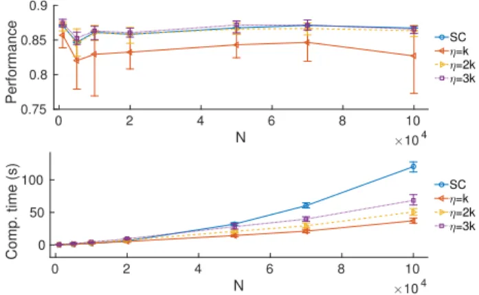
Fig. 3. Average (and 10 and 90% quantiles) performance (top) and computation time (bottom) over 20 realisations of the Gaussian dataset illustrated in Fig. 1 for the classical spectral clustering algorithm (SC), and our proposition for

η=k,2kand3k.

(right) shows one recovered labeling fork= 10.

We compare our method vs. classical spectral clustering in Figure 3 in terms of performance and time of computation. We note that forη= 2kandη= 3k, our method performs as well as the classical algorithm; while forη =k, on the other hand, the number of random signals becomes insufficient as we observe the recovery starting to fail. Up toN '4.104, the computation time is slightly faster with the classical algo-rithm. But asN increases, the classical algorithm’s comput-ing time increases significantly faster than our proposition’s: forN = 105_{for instance, computation time is 2 (resp. 2.5,} 3) times faster when one usesη = 3k(resp. 2k,k) random signals than the classical algorithm.

6. CONCLUSION

We propose a new method that paves the way to alternative spectral clustering methods bypassing the usual computa-tional bottleneck of extracting the Laplacian’s firstk eigen-vectors. We take advantage of the fast graph low-pass graph filtering of a few random vectors to estimate the spectral clustering distance. The use of random vectors makes our algorithm stochastic, which in turn enables us to define a stability measureγfor anyk: scales of interest maximizeγ. Results on synthetic data show that our method is scalable and forη_&k, one has the same performance as with the clas-sical spectral algorithm while reducing the time complexity by a few factors.

We prooved that the error on the estimation of the dis-tanceDijis well controlled, but the question of how such an

error propagates on the estimation of the clusters themselves is open. Moreover, the impact of the errorδof the polyno-mial approximation on the rest of the algorithm is still largely unknown and matter of future work.

7. REFERENCES

[1] D. Ramasamy and U. Madhow, “Compressive spec-tral embedding: sidestepping the SVD,” in Advances

in Neural Information Processing Systems, Dec 2015,

pp. 550–558.

[2] U. von Luxburg, “A tutorial on spectral clustering,”

Statistics and Computing, vol. 17, no. 4, pp. 395–416, 2007.

[3] H. Jia, S. Ding, X. Xu, and R. Nie, “The latest research progress on spectral clustering,”Neural Computing and Applications, vol. 24, no. 7-8, pp. 1477–1486, 2014. [4] J. Lei and A. Rinaldo, “Consistency of spectral

cluster-ing in stochastic block models,” Ann. Statist., vol. 43, no. 1, pp. 215–237, 02 2015.

[5] U. Kang, B. Meeder, E.E. Papalexakis, and C. Faloutsos, “Heigen: Spectral analysis for billion-scale graphs,”

Knowledge and Data Engineering, IEEE Transactions on, vol. 26, no. 2, pp. 350–362, Feb 2014.

[6] A. K. Jain, M. N. Murty, and P. J. Flynn, “Data cluster-ing: A review,” ACM Comput. Surv., vol. 31, no. 3, pp. 264–323, Sept. 1999.

[7] S. Ben-David, U. von Luxburg, and D. Pl, “A sober look at clustering stability,” inLearning Theory, Gbor Lugosi and HansUlrich Simon, Eds., vol. 4005 ofLecture Notes in Computer Science, pp. 5–19. Springer Berlin Heidel-berg, 2006.

[8] A. Sandryhaila and J.M.F. Moura, “Big data analysis with signal processing on graphs: Representation and processing of massive data sets with irregular structure,”

Signal Processing Magazine, IEEE, vol. 31, no. 5, pp. 80–90, Sept 2014.

[9] D.I. Shuman, S.K. Narang, P. Frossard, A. Ortega, and P. Vandergheynst, “The emerging field of signal pro-cessing on graphs: Extending high-dimensional data analysis to networks and other irregular domains,” Sig-nal Processing Magazine, IEEE, vol. 30, no. 3, pp. 83– 98, May 2013.

[10] N. Tremblay and P. Borgnat, “Graph wavelets for mul-tiscale community mining,” Signal Processing, IEEE

Transactions on, vol. 62, no. 20, pp. 5227–5239, Oct

2014.

[11] N. Tremblay and P. Borgnat, “Multiscale community mining in networks using the graph wavelet transform of random vectors,” inGlobal Conference on Signal and

Information Processing (GlobalSIP), 2013 IEEE, Dec

2013, pp. 463–466.

[12] S. Roux, N. Tremblay, P. Borgnat, P. Abry, H. Wendt, and P. Messier, “Multiscale anisotropic texture unsuper-vised clustering for photographic paper,” in 7th IEEE International Workshop on Information Forensics and Security (WIFS), 2015.

[13] D.I. Shuman, P. Vandergheynst, and P. Frossard, “Chebyshev polynomial approximation for distributed signal processing,” inDistributed Computing in Sensor Systems and Workshops (DCOSS), 2011 International Conference on, June 2011, pp. 1–8.

[14] A.Y. Ng, M.I. Jordan, Y. Weiss, et al., “On spectral clus-tering: Analysis and an algorithm,” Advances in neu-ral information processing systems, vol. 2, pp. 849–856, 2002.

[15] F.R.K. Chung,Spectral graph theory, Number 92. Amer Mathematical Society, 1997.

[16] A. Sandryhaila and J.M.F. Moura, “Discrete signal pro-cessing on graphs,” Signal Processing, IEEE Transac-tions on, vol. 61, no. 7, pp. 1644–1656, April 2013. [17] T. Hastie, R. Tibshirani, J. Friedman, and J. Franklin,

“The elements of statistical learning: data mining, infer-ence and prediction,” The Mathematical Intelligencer, vol. 27, no. 2, pp. 83–85, 2005.

[18] D. Achlioptas, “Database-friendly random projections: Johnson-lindenstrauss with binary coins,” Journal of Computer and System Sciences, vol. 66, no. 4, pp. 671 – 687, 2003, Special Issue on{PODS}2001.

[19] D.I. Shuman, C. Wiesmeyr, N. Holighaus, and P. Van-dergheynst, “Spectrum-adapted tight graph wavelet and vertex-frequency frames,” Signal Processing, IEEE Transactions on, vol. PP, no. 99, pp. 1–1, 2015.

[20] L.N. Trefethen and D. Bau III, Numerical linear alge-bra, vol. 50, Siam, 1997.

[21] R. Xu and D. Wunsch II, “Survey of clustering algo-rithms,” Neural Networks, IEEE Transactions on, vol. 16, no. 3, pp. 645–678, May 2005.

[22] A. Ben-Hur, A. Elisseeff, and I. Guyon, “A stabil-ity based method for discovering structure in clustered data.,” in Pacific symposium on biocomputing. World Scientific, 2002, vol. 7, pp. 6–17.

[23] L. Hubert and P. Arabie, “Comparing partitions,” Jour-nal of classification, vol. 2, no. 1, pp. 193–218, 1985. [24] N. Perraudin, J. Paratte, D. Shuman, V. Kalofolias,

P. Vandergheynst, and D.K. Hammond, “Gspbox: A toolbox for signal processing on graphs,”arXiv preprint arXiv:1408.5781, 2014.