Soil Modelling Techniques

(1)

Published online December 30, 2012 (http://www.sciencepublishinggroup.com/j/ijmsa) doi: 10.11648/j.ijmsa.20120101.12

Soil modelling techniques

Gary Gilbert

Dept. name of organization, City, Country

Email address:

To cite this article:

Gary Gilbert. Soil Modelling Techniques, International Journal of Materials Science and Applications. Vol. 1, No. 1, 2012, pp. 8-13. doi: 10.11648/j.ijmsa.20120101.12

Abstract:

The main objective of grounding electrical systems is to provide a suitably low resistance connection to the substation above it the low resistance is needed to limit the potential rise of the substation from the potential of the sur-rounding earth. This potential rise must be limited so that there is no danger to anyone standing on ground but touching, for example, the substation fence. In order to ensure that the ground potential rise, and touch and step voltages, an accurate soil model are needed to perform calculations that ensures that the resistance of the grounding grid through the earth is sufficiently low. This soil model comes from the tested soil structure at the proposed grid location. This paper provides a literature survey of the various soil testing methods and soil modeling. The paper is divided into 2 parts: Part 1 describes the current soil measurement techniques; Part 2 examines the model construction of the uniform and two layer soil structures, and the short comings of the current modeling techniques.

Keywords:

Soil Model, Sunde’s Curves, High Voltage Substation Grounding

1. Introduction

Resistance is the property of a conductor that opposes electric current flow when a voltage is applied across the two ends of a linear conductor. The unit of measure for resistance is the Ohm (Ω), and the commonly used symbol is R. The resistance of a conductor depends on the atomic structure of the material or its resistivity (measured in Ohm.m or Ω.m), and it can be calculated from the resistivity of the conductor using the standard definition of (1):

A

L

R

=

ρ

*

(1)

where: ρ is the resistivity (Ω.m) of the conductor material

L is the length of the conductor (m)

A is thecross sectional Area (m2)

Equivalent to (1), soil resistivity can be defined as the resistance between the opposite sides of a cube of soil with a side dimension of one meter. Soil resistivity values in vary widely, depending on the type of terrain; e.g., silt on a ri-verbank may have a resistivity value around 1.5 Ω.m, whe-reas dry sand or granite in mountainous country may have values higher than 10,000 Ω.m. The factors that affect re-sistivity may be summarized as follows [1]:

Type of earth (e.g., clay, loam, sandstone, granite). Stratification of layers of different types of soil (e.g.,

loam backfill on a clay base).

Moisture content: resistivity may fall rapidly as the moisture content is increased, but after a value of about 20%, the rate is much less. Soil with moisture content greater than 40% is rarely encountered. Temperature: above the freezing point, the effect of temperature on earth resistivity is negligible. Chemical composition and concentration of dis-solved salts. Presence of metal and concrete pipes, tanks, large slabs, cable ducts, rail tracks, or metal pipes. Figure 1 shows how resistivity varies with salt content, moisture, and temperature.

It is found that earth resistivity varies from 0.01 to 1 Ω.m for sea water, and up to 109 Ω.m for sandstone Figure 1.1. The resistivity of the earth increases slowly with decreasing temperatures from 25oC, while for temperatures below 0oC, the resistivity increases rapidly. In frozen soil, as in the surface layer in winter, the resistivity may be exceptionally high. Table 1 shows the resistivity values for various soils and rocks that might occur in different grounding system designs.

(2)

International Journal of Materials Science and Applications 2012, 1(1):8-13 9

layers, each having a different resistivity, in which case the soil is said to be non-uniform. Lateral changes may also occur, but, in general, these changes are gradual and neg-ligible, at least in the vicinity of a site where a grid is to be installed. In most cases, measurements will show that the resistivity, ρ, is mainly a function of depth. The interpreta-tion of the measurements consists of establishing a simple equivalent function to yield the best approximation of soil resistivity’s to determine the layer model.

Figure 1. Soil Resistivity Variations [1].

Table 1. Resistivity values for several types of soils and water 25°C [2].

Type of Soil or Water

Typical

Resistivity (Ω.m) Usual Limit (Ω.m) Sea water 2 0.1 to 10

Clay 40 8 to 70

Ground well and

spring water 50 10 to 150 Clay and sand mixtures 100 4 to 300 Shale, slates, sandstone, etc. 120 10 to 100 Peat, loam, and mud 150 5 to 250 Lake and brook water 250 100 to 400 Sand 2000 200 to 3000 Moraine gravel 3000 40 to 10000 Ridge gravel 15000 3000 to 30000 Granite 25000 10000 to 50000 Ice 100000 10000 to 100000

In the case of station grounding systems, a two-layer soil model (Figure 1.2) has been found to be a good approxima-tion of the soil structure for ground system designs [2].

Figure 2. Two-Layer Soil Model.

2. Review of Existing Soil Resistivity

Measurement Procedures

Soil resistivity measurements are used to obtain a set of measurements that may be used to yield an equivalent soil model for the electrical performance of the earth. The results, however, may be unrealistic if adequate background inves-tigation is not made prior to the measurement. The back-ground investigation includes data related to the presence of nearby metallic structures, as well as the geological, geo-graphical, and meteorological information of the area. For instance, geological data regarding strata types and thick-nesses would give an indication of the water retention properties of the upper layers and therefore their expected variation in resistivity between the layers; then a comparison of recent rainfall data against the seasonal average would indicate if resistivity results found are realistic.” Such background investigation is usually included as a part of the soil measurement procedure.

Soil resistivity measurements are made by injecting cur-rent into the earth between two outer curcur-rent probes and measuring the resulting voltage between two inner potential probes placed along the same straight line. When the adja-cent current and potential probes are close together, the measured soil resistivity is indicative of local surface soil characteristics. When the probes are far apart, the measured soil resistivity is indicative of average deep soil characte-ristics throughout a much larger area. In principle, soil re-sistivity measurements are made using spacing (between adjacent current and potential probes) that are, at least, on the same order as the maximum size of the grounding system (or systems) under study. It is, however, preferable to extend the measurement traverses to several times the maximum grounding system dimension, where possible. Often, it will be found that the maximum probe spacing is governed by other considerations, such as the maximum area of the available land which is clear of interfering bare buried conductors.

2.1. Soil Resistivity Measurement Procedure

Factors such as maximum probe depth, lengths of cables required, efficiency of the measuring technique, cost (de-termined by time and the size of the survey crew), and ease

1

ρ

0 :

ρ

=

Air

(3)

of interpretation of the data must be considered when se-lecting the test type. Three common test types are the Wenner 4-Probe Method, Schlumberger Array, and the Driven Rod (3-Probe) Method. These methods will be dis-cussed below. In homogenous isotropic earth, the resistivity will be constant; however, if the earth is non-homogenous and the electrode spacing is varied, a different value of re-sistivity will be found for each surface measurement. This value of soil resistivity is referred to as the apparent resis-tivity, ρa. For the three common test types, the measurement

techniques and the test methods’ equations will be presented.

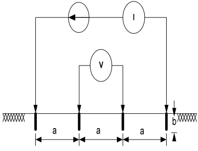
2.1.1. Wenner Array

In the Wenner method (See Figure 2.3), all four probes are moved for each test, with the spacing between each adjacent pair remaining the same [1]. In the Wenner 4-probe method, it is possible to measure the average resistivity of the soil between the two center probes to a depth equal to the probe spacing between adjacent probes. If the probe spacing is increased, then the average soil resistivity is measured to a greater depth. If the average resistivity increases as the probe spacing increases, there is a region of soil having resistivity at the greater depth.

Figure 3. Wenner four-probe method.

Equation 2.1, determines the apparent resistivity based on the surface measurements as shown in Figure 3 if the pene-tration of the probe, b, is small compared to the spacing of the four probes (i.e., a>106) [1].

aR

a π

ρ =2 (2)

where: ρa is the apparent resistivity (Ω.m)

a is the probe spacing (m)

R is the measured resistance (Ω)

If the ratio between the penetrations of the probe b is small compared to the spacing of the four probes, then (2.3) is used. This is a curve fitted equation, developed by Wen-ner.

2 2 2 2

4

2

1

4 b

a

b

a

aR

a

+

−

+

=

π

ρ

(3)

2.1.2. Schlumberger Array

The Schlumberger array (Figure 2.4) requires that the outer probes be moved four or five times for each position of the inner probes [1]. The reduction in the number of probe moves also reduces the effect of lateral variation in the test results. Considerable time savings can be achieved by using this method, since there will less probe placements than required by the Wenner method, with similar results. The minimum spacing accessible is in the order of 10m (for a 0.5 m inner spacing), thereby necessitating the use of the Wen-ner configuration for smaller spacing. Lower voltage read-ings are obtained when using Schlumberger arrays. This may be a critical problem where the depth required to be tested is beyond the capability of the test equipment or the voltage readings are too small to be useful.

The Schlumberger array is more complex, with the spacing between the current probes not equal to the spacing between the potential probes. Equation 2.4 determines the apparent resistivity based on the surface measurements as shown in Figure 4.

Figure 4. Schlumberger Array.

M

R

L

a

2

π

ρ

=

(4)

L is the distance from the center line to the outer probes (m)

M is the distance from the center line to the inner probes (m)

R is the measured resistance (Ω)

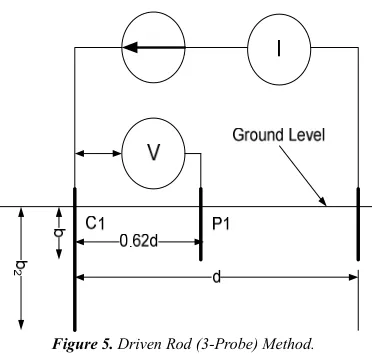
2.1.3. Driven Rod Method

(4)

Figure 5. Driven Rod (3-Probe) Method.

Equation 2.5 determines the apparent resistivity based on the surface measurements as shown in Figure 4.













=

d

b

R

b

a

2 2

2 ln

2 π

ρ

(5)

b2 is the length of the driven rod in contact with the earth (m)

d is the spacing between the current probes (m) R is the measured resistance (Ω)

Significant tests from Ohio State have demonstrated all of the measurement techniques above yield similar results [3]. In the research, however, conducted by Ohio State, the measurement spacing began to play a common factor in all of the measurement techniques. It was determined that there must be significant changes in the measurement spacings. For example, an increase of 1m to 2m would be considered significant, while an increase 1.1m to 1.2m would not.

2.1.4. Spacing Range

The range of spacings recommended in [3] includes ac-curate close probe spacings (≤1 m), which are required to determine the upper layer resistivity, used in calculating the step and touch voltages, to spacings larger than the radius or diagonal dimension of the proposed earth grid. The larger spacings are used in the calculation of remote voltage gra-dients and grid impedances. Measurements at very large spacings often present considerable problems. Such prob-lems include inductive coupling, insufficient resolution of the test set, and physical.

3. Determination of the Soil Structure

This part of the paper introduces the uniform soil model and then a numerical solution for the two layer soil model, based on the soil parameters obtained through testing me-thods discussed earlier.

3.1. Uniform Soil Model

Soil characteristics can be approximated from surface measurements, which provide a resistivity of the soil, ρa. If

ρa is constant for various probe spacings, it is an indication

that the earth at the measurement site is fairly uniform; otherwise, a two-layer model should be used. Figure 3.6 represents the soil structure for the uniform soil model.

Figure 6. Uniform Soil Model.

The resistivity of a uniform soil model is determined by either (2) or (3), depending on whether the penetration of the probe, b, is small compared to the spacing of the four probes, and assumes the soil resistivity is uniform in nature to an infinite depth. After taking all of the surface measurements and determining the various resistivities at the substation location, an overall ρa for the grounding system can be

de-termined. The IEEE 80-2000 standard [1] offers two equa-tions for this calculation. The first equation is determined by an averaging of all of the measured values

Where

n

n a a

a a a

) ( ) 3 ( ) 2 ( ) 1

(

ρ

₌

+

⋯

(6)

are the measured apparent resistivity data obtained at different spacings by the methods discussed earlier, and n is the total number of measurements. The other equation that can be used is the following:

2

(min) (max) a a

a

ρ

=

+

(7)

3.2. Two-Layer Soil Model

Typically, the observed resistivity’s vary when plotted as a function of the probe spacing. Large variations in probe spacing (a variance of greater than 30%) indicate that the earth is non-uniform, and a two-layer soil model must be used. Using a single-layer model in such a situation has been shown to cause significant error [4].

Figure 2 represents the two layered soil model, which has an upper layer of a finite depth, h, and resistivity, ρ1, over a

lower layer of infinite depth and resistivity, ρ2. The difficulty

in using this model is the mathematical determination of the depth of layer one, due to the numerous variations in the structure and properties of the earth. This research will in-troduce a new technique that can be used in the determina-tion of h.

(5)

be grouped into two categories: empirica

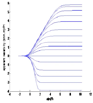
Empirical methods are typically developed through a co bination of interpolation and field measurements. Sunde [5] first proposed a graphical method to approximate a two-layer soil model, based on the interpretation of a series of curves which are commonly called the “Sunde curves.” The graph in Figure 3.7, which is based on the Wenner four-pin test method, shows those curves, which are repr duced from Figure 6 of Sunde’s text [5].

Figure 7. Sunde Curves for Two-Layer Soil Structure From

Parameters ρ1 and ρ2 are obtained by inspection of resi

tivity measurements. The third parameter,

Sunde’s graphical method, which is explained in detail in the IEEE Standard 80, along with an example [1]

Curve allow for a rough approximation of the soil model parameters without the use of a computer or sophisticated equations and provided designers with a fundamental process to determine the soil model for many years. Due to the inaccuracies of the Sunde curves, as this method relies on the visual interpolation of the Sunde curves to determine the three soil model parameters, researchers were led to further Sunde’s work. To this end, in [6],

Blattner found that the empirical solution

Sunde curves provided a rough approximation of the resi tivities and depth of the first layer in the two

however, they worked towards a more rigorous solution. The researchers developed a duplicate of the Sunde curves to provide a benchmark for a logarithmic curve

proach to determine the parameters [3]. The shortcoming of this method was that it was not an analytical solution, and relied on the Sunde curves themselves.

Seedher and Arora [7] introduced smoothing consta enhance the equations of [1] which reduced the errors of both Sunde’s and Dawalibi methods. The smoothing fun tion proposed in [7] allowed for small fluctuations in the uniform soil approximation introduced by Sunde, but the be grouped into two categories: empirical or analytical. Empirical methods are typically developed through a com-bination of interpolation and field measurements. Sunde [5] first proposed a graphical method to approximate a layer soil model, based on the interpretation of a series hich are commonly called the “Sunde curves.” 7, which is based on the Wenner pin test method, shows those curves, which are repro-duced from Figure 6 of Sunde’s text [5].

Layer Soil Structure From Image Theory.

are obtained by inspection of resis-The third parameter, h, is obtained by Sunde’s graphical method, which is explained in detail in the IEEE Standard 80, along with an example [1]. The Sunde Curve allow for a rough approximation of the soil model parameters without the use of a computer or sophisticated equations and provided designers with a fundamental process to determine the soil model for many years. Due to he Sunde curves, as this method relies on the visual interpolation of the Sunde curves to determine the three soil model parameters, researchers were led to further Sunde’s work. To this end, in [6], Dawalibi and found that the empirical solution found using the Sunde curves provided a rough approximation of the resis-tivities and depth of the first layer in the two-layer model; however, they worked towards a more rigorous solution. The researchers developed a duplicate of the Sunde curves to e a benchmark for a logarithmic curve-matching ap-proach to determine the parameters [3]. The shortcoming of this method was that it was not an analytical solution, and

Seedher and Arora [7] introduced smoothing constants to enhance the equations of [1] which reduced the errors of both Sunde’s and Dawalibi methods. The smoothing func-tion proposed in [7] allowed for small fluctuafunc-tions in the uniform soil approximation introduced by Sunde, but the

fundamental equations for modeling remained the same, as this method relied on the original Sunde’s curves. In [8], del Alamo compared several techniques used in the estimation of the soil parameters and improved on the evaluation of the parameters by introducing a Newton optimiz

Although there were reductions in the errors between the actual soil structure and that of the calculation due to the optimization process, the technique was limited by the use of equations that were formulated by the Sunde’s curves and the starting conditions of the optimization process itself. While the soil model parameter errors were reduced, the fundamental basis of the use of images remained the same in that the Sunde curves were used. More recently, Gonos and Stathopulos [9] successfully used a genetic algorithm to reduce errors in the soil model for the two

The technique developed by Gonos and Stathopoulos i proved only the optimization process itself, and did not eliminate the use of complex images to determine the s model parameters.

All of the algorithms mentioned above effectively match Sunde’s curves, which are generated from multiple complex images (in the actual physical space or its equivalent spectral space). The formula of the multiple complex images is an infinite series which is complicated and not easy to unde stand in its behaviour. Easy understanding would enhance the confidence of the constructed soil model, and lead to better grounding grid designs, and possible design extension to three layer soils. By changing the existing method of Sunde, researchers have found that an optimization process is required to improve the error of the constructed soil model. It would be helpful, therefore, if a simple analytical formula for the determination of the soil

the use of images could be found.

6. Conclusion

This paper provided a discussion of the parameters that affect grounding grid design, the importance of a good soil model, and a survey of existing techniques used to finds those models. One of the commonly used methods is the graphical Sunde which is based on complex i ages.Researchers have advanced some of the original tec nique developed by the Sunde curves for comparison during calculations; however, there has been little effort in mining the soil model directly from the field measurements themselves. The next paper provides a new method to d termine the soil model parameters directly from field me surements, based on equations that replace the Sunde curves and the use techniques using multiple complex im

References

[1] The Institute of Electrical and Electronic Engineers, Inc. (2000). IEEE Guide for Safety in AC Substation Grounding. New York: Publisher.

[2] Dawalibi, F.P. and D. Mukhedkar. “ Optimum design of r modeling remained the same, as this method relied on the original Sunde’s curves. In [8], del Alamo compared several techniques used in the estimation of the soil parameters and improved on the evaluation of the parameters by introducing a Newton optimization process. Although there were reductions in the errors between the actual soil structure and that of the calculation due to the optimization process, the technique was limited by the use of equations that were formulated by the Sunde’s curves and starting conditions of the optimization process itself. While the soil model parameter errors were reduced, the fundamental basis of the use of images remained the same in that the Sunde curves were used. More recently, Gonos and ly used a genetic algorithm to reduce errors in the soil model for the two-layer soil model. The technique developed by Gonos and Stathopoulos im-proved only the optimization process itself, and did not eliminate the use of complex images to determine the soil

All of the algorithms mentioned above effectively match Sunde’s curves, which are generated from multiple complex images (in the actual physical space or its equivalent spectral The formula of the multiple complex images is an infinite series which is complicated and not easy to under-stand in its behaviour. Easy underunder-standing would enhance the confidence of the constructed soil model, and lead to better grounding grid designs, and possible design extension By changing the existing method of Sunde, researchers have found that an optimization process is required to improve the error of the constructed soil model. It would be helpful, therefore, if a simple analytical formula for the determination of the soil model parameters without

e use of images could be found.

This paper provided a discussion of the parameters that affect grounding grid design, the importance of a good soil model, and a survey of existing techniques used to finds ls. One of the commonly used methods is the graphical Sunde which is based on complex im-ages.Researchers have advanced some of the original tech-nique developed by the Sunde curves for comparison during calculations; however, there has been little effort in deter-mining the soil model directly from the field measurements themselves. The next paper provides a new method to de-termine the soil model parameters directly from field mea-surements, based on equations that replace the Sunde curves

es using multiple complex images.

The Institute of Electrical and Electronic Engineers, Inc. (2000). IEEE Guide for Safety in AC Substation Grounding.

(6)

substation grounding in two-layer earth model—Part I ana-lytical study,” IEEE Transactions in Power Systems Appli-cations, Vol. 94, pp. 252-261, March, 1975.

[3] Ma, J., F. P. Dawalibi, and R. D. Southey. “On the equiva-lence of uniform and two-layer soils to multilayer soils in the analysis of grounding systems,” in Proceedings on the Insti-tute Electrical Engineers—Generation, Transmission and Distribution, 1996, pp. 49-55.

[4] Dawalibi, F.P. and N. Barbeit. “ Measurements and compu-tations of the performance of grounding systems buried in multilayer soils,” IEEE Transactions on Power Delivery, Vol. 6, pp. 1483-1490, October, 1991.

[5] Sunde, E. D., Earth conduction effects in transmission sys-tems, New York: McMillan, 1968.

[6] Dawalibi, F. and C.J. Blattner. “Earth resistivity measurement

interpolation techniques,” IEEE Transactions on Power Ap-paratus and Systems, Vol. PAS-103, pp. 374-382, February, 1984.

[7] Chow, Y.L. and M.M.A. Salama. “A simplified method for calculating the substation grounding grid resistance, “ IEEE Transactions on Power Delivery , Vol. 9, pp. 736-742, April, 1994.

[8] Nekhoul, B., P. Labie, F.X. Zgainski, and G. Meunier. “Cal-culating the impedance of a grounding system,” IEEE Transactions on Magnetics, Vol. 32, pp. 1509-1512, May, 1996.