Computer Simulation-Based Designs for Industrial Engineering Experiments

http://www.sciencepublishinggroup.com/j/sjams doi: 10.11648/j.sjams.20180603.12

ISSN: 2376-9491 (Print); ISSN: 2376-9513 (Online)

Computer Simulation-Based Designs for Industrial

Engineering Experiments

Dongyu Zhou, Weihua Guo, Hengzhen Huang

*

College of Mathematics and Statistics, Guangxi Normal University, Guilin, China

Email address:

*_{Corresponding author}

To cite this article:

Dongyu Zhou, Weihua Guo, Hengzhen Huang. Computer Simulation-Based Designs for Industrial Engineering Experiments. Science Journal of Applied Mathematics and Statistics. Vol. 6, No. 3, 2018, pp. 74-80. doi: 10.11648/j.sjams.20180603.12

Received: April 27, 2018; Accepted: May 19, 2018; Published: June 7, 2018

Abstract:

Computer simulations have been receiving a lot of attention in industrial engineering as the rapid growth in computer power and numerical techniques. In contrast to physical experiments which are usually carried out in factories, laboratories or fields, computer simulations can save considerable time and cost. From the statistical perspective, the current research work about computer simulations is mostly focusing on modeling the relationship between the output variable from the simulator and the input variables set by the experimenter. However, an experimental design with careful selection of the values of the input variables can significantly affect the quality of the statistical model. Specifically, prediction on the edge area of the experimental domain, which is extremely critical for an industrial engineering experiment often suffers from inadequate data information because the design points usually do not well cover the edge area of the experimental domain. To address this issue, a new type of design, called semi-LHD is proposed in this paper. Such a design type has the following appealing properties: (1) it encompasses a Latin hypercube design as a sub-design so that the design points are uniformly scattered over the interior of the design region; and (2) it possesses some extra marginal design points which are close to the edge so that the prediction accuracy on the edge area of the experimental domain is fully taken into account. Detailed algorithms for finding the marginal design points and how to construct the proposed semi-LHDs are given. Numerical comparisons between the proposed semi-LHDs with the commonly-used Latin hypercube designs, in terms of prediction accuracy, are illustrated through simulation studies. It turns out that the proposed semi-LHDs yield desirable prediction accuracy not only in the interior but also on the edge area of the experimental domain, so they are recommended as the experimental designs for simulation-based industrial engineering experiments.

Keywords:

Computer Experiments, Design of Experiments, Gaussian Process Model, Kriging, Latin Hypercube Design

1. Introduction

Computer experiments are becoming widely used in industrial engineering where computational methods are used to simulate the real-world phenomena (see, for example, references [1-7]). Most computer experiments for industrial engineering are unique in that the response has no random-error component. That is, replicates of the same inputs to the computer code will yield the same response. Since a computer experiment is typically treated as a black-box and is time demanding, the experimental design should be chosen judiciously and explore the experimental domain as thoroughly as possible. To this end, Mckay, Beckman and

Conover [8] first proposed the Latin hypercube designs (LHDs) which possess the property that when projected onto any one dimension, they achieve maximum stratification. LHDs are the most popular designs for computer-based industrial engineering experiments and have enjoyed lots of development (see, for example, references [6, 7, 9-12]).

detailed treatment of this topic, please refer to references [6, 7]. Most of the existing work are paying attentions on modeling methods, while a design with careful planning can significantly affect the prediction accuracy of the model. When predicting the response at an unobserved site located in the interior of the design region, information is often sufficiently received from the design points around it. However, when the unobserved site is located on the edge of the design region, inadequate information may be received because the relatively small number of design points around it. As a result, the prediction accuracy on the edge of the design region may be poor, especially for industrial engineering experiments. The engine block and head joint sealing assembly experiment, the robot arm experiment and the integrated circuit experiment described by [1] are some good examples of this and very few experimental designs have been proposed to address this issue.

Motivated by the aforementioned issue, a new design type called semi-LHD is proposed for computer-based industrial engineering experiments which pays extra attention to the edge area of the experimental domain. A semi-LHD adds extra points to the marginal points of an LHD so that the proposed design inherits the space-filling property of the LHD. Furthermore, the proposed semi-LHD helps to increase the prediction accuracy on the edge while not deteriorating the overall prediction accuracy. Methods for finding marginal points and choosing the added points are systematically proposed, which are the central contributions of this work.

The remainder of this paper is organized as follows. Section 2 provides useful definitions and notations. Section 3 presents the design construction method and gives some numerical examples that simulate industrial engineering experiments. Concluding remarks in Section 4 close this paper.

2. Definitions and Notations

In this section, some useful definitions and notation will be given. A Latin hypercube design (LHD) is a n×p matrix, denoted by LHD (n, p) in which the number of levels in each column equals to the sample size and the levels are equally spaced. Without loss of generality, suppose that the design region is the unit cube[0,1]p. That is, when the design points of an n-run LHD are projected on each dimension, there is exactly one point falling into each of the n equally spaced intervals on [0, 1]. In general, a random LHD can be constructed as follows. Let A=(a_{ij n p}) _× be an n×p matrix each column of which is a random permutation of (1, 2,..., n), and the columns are generated independently.

Via A, construct an n×p matrix D=(d_{ij n p}) _× where

, ij ij ij

a u d

n

−

= (1)

and uijis a random number drawn from U(0, 1) and aijand ij

u are independent, i=1,...n, j=1,...p. Then D is a random LHD.

One primary goal of a computer experiment is to establish an emulator (also called a metamodel) which can capture the relationship between the inputs and the output of the computer code. In this paper the most commonly-used model, the Gaussian process model (see references [6, 7, 16]) is considered. Given an input x∈[0,1]p, the response y x( )is modeled as

( ) ( ) ' ( , ),

y x = f x β+Z x Θ (2)

where f x( )=( ( ),...,f x1 f xq( )) ' are some known functions

defined on the design region,

β

=(

β

₁,...,

β

_q) 'is a vector of unknown parameters to be estimated and Z x( , )Θ assumed to be a realization of a stationary Gaussian process with zero mean, variance σ2and a vector of correlation parameters

1

( ,...,

θ

θ

_p) '.

Θ = Given two different inputs x₁=(x₁₁,...,x_1p)

2

1 2 1 2

[ ( ), ( )] ( | ),

Cov y x y x =

σ

r x −x Θ

where r( |⋅ Θ) is the correlation function defined by the parameter Θ_.The most commonly-used correlation function is the Gaussian correlation function, which is given by

2

1 2 1 2 1 2

1

( | ) [ ( ), ( )] exp{ ( ) },

p

i i i i

r x x corr y x y x θ x x

=

− Θ = = −

_∑

− (3)

where θ_i's are required to be positive. Throughout this paper, this correlation function is used since it is infinitely differentiable which is favorable in applications for industrial engineering [3].

A popular method for analyzing the model in (2) is through kriging [7]. Given a design of n inputs D=( ,...,x₁' x_n') on

[0,1]p with the corresponding response vector

1

( ( ),..., ( _n)) '

y= y x y x , according to the Gaussian process assumption, y follows the following multivariate normal distribution

2

( , ),

∼

y MN F

β σ

R

where F=( ( ),..., (f x1 f xn)) ',R=( )rij n n× is the n n×

correlation matrix with rij being r x( i−xj| )Θ defined in (3).

The negative log-likelihood of y is proportional to

2 1 2

log( ) log(| |) ( ) ' ( ) / ,

n

σ

+ R + −y F

β

R− y F−

β σ

(4)

1 1 1 ( 'F R F) F R y' ,

β∧ ₌ − − − ₍₅₎

2 _{(y F ) 'R} 1_{(y F ) / ,n}

σ

∧ _{= −}

β

− ₋

β

(6)

respectively. It is easy to see that β

∧

,σ2

∧

and Rare functions of the parameter Θ . Plug the MLEs of β and σ2 into formula (4), the MLE of Θis then given by

2

arg min ( log(n

σ

) log(|R|)).

∧ ∧

Θ

Θ = + (7)

There are several optimization algorithms available to solve the problem in (7), see Fang, Li and Sudjianto [1] for

details. Plug

∧

Θback into Eqs. (5) and (6), the best linear unbiased predictor (BLUP) of the response yat an untried point x*is given by

1 ^

* *

( ) ( ) ' r ' ( ),

y x f x β R y Fβ

−

∧ ∧ ∧

= + − (8)

where r ( (r x* x₁) | ),..., (r x* x_n) | )) '

∧ ∧

= − Θ − Θ and R∧ is the

n n× correlation matrix with the ( , )i j th entry being

( _{i j}) | )

r x −x Θ∧ . It is easy to verify that predictor (8) interpolates the response at any observed point x_i, which is a desired property for deterministic computer experiments.

3. The Methodology

3.1. The Design Construction Method

In this section an easy-to-implement method is presented to construct a new type of design called semi Latin hypercube design (semi-LHD). This design type is useful for predicting the responses at untried points which are specially located on or close to the edge of the experimental region. As for the points far away from the edge, the proposed design can also yield good prediction accuracy. The main idea of the proposed design is to add points to an existing LHD, thus the resulting design contains an LHD as a subdesign.

Suppose an n-run semi-LHD is to be constructed, the number of runs of the built-in LHD n₀(<n) is determined according to the needs of the experiment. Determine the parameter mwhich is the number of “marginal points” of the built-in LHD. Given n, n₀ and m, the general framework of the proposed design construction method is presented as follows.

Display 1 (Framework of the construction of semi-LHDs).

Step 1. Construct an LHD (n₀ , p ), denoted as D₁. Without loss of generality, let

0 1 ( ,...,1 n ) '

D = x x , where

0 1,..., n

x x are rows (points) of D₁.

Step 2. Fori=1,...,n₀,calculate the average distance from

i

x to the remaining points in D₁, denoted by a_i . Let

0 1

( ,..., _n ) '.

a= a a Sort the elements in vector a in descending

order and denote the resulting vector by

0

* * *

1

( ,..., _n ) '.

a = a a

Rearrange the rows in D₁ by a* and denote the resulting design by D₁*.

Step 3. Let the first mrows of D₁*form a subdesign d₁*. For each point in d₁*, add lpoints around it following a pre-specified regulation, where lis the smallest integer satisfying

0 ml≥ −n n .

Step 4. Combine the ml points added in the previous step to form a design E*. Let D*=(D₁*',E*') '.If ml= −n n₀,

*

D=D is the desired design. If ml> −n n₀ , delete

0

( )

ml− −n n points from E*following some rule and still denote the resulting array by E*. Then D=(D₁*',E*') 'is the desired design.

The steps in Display 1 are given in a general manner, hereafter the details surrounding the framework are presented. As alluded to earlier, n₀is determined according to the experimental needs. If n is not large, say

0

50, / 2 2 / 3

n≤ n ≤n ≤ n is recommended as a standard choice so that at least a small number of design points can be added; if n is large, n₀ can be a relative large portion of n. In Step 1 of Display 1, a random LHD or a maximin distance LHD with sample size n₀can be used. Other optimal LHDs could also be considered at this step. For simplicity, a random LHD is used throughout this paper. In Step 2, the average distance a_i from x_i of D₁ to the remaining points in D₁ is calculated by

0

2

0 1, 1

1

( ) .

1

n p

i ij kj

k k i j

a x x

n _{= ≠ =}

= −

−

∑ ∑

(9)

The design points in D₁*in Step 2 is ordered so that the first row has the largest average distance from the others, the second row has the second largest average distance and so on. It is clear that points with relatively large average distance are located near the edge of the design region and far from the other points.

Parameter m in Step 3 is another value determined according to the practical needs. In applications, m≈n₀/ 4

may be used as a standard choice, which represents the belief that about a quarter of the design points of the built-LHD are treated as the marginal points. The first m rows of D₁* are thought to be marginal points since each of them has relatively large distance from the other points in D₁*. With a

little abuse of notation, denote d₁*=( ,...,x₁ x_m) ' . where

' ' 1,..., m

1

( ,..., ) ', 1,..., .

i i ip

x = x x i= m In Step 3, l points are added

around each point in d1*. An algorithm for how to add the

points is given as follows. Algorithm 1.

Step 1. For i=1,..., ,m j=1,...,land k=1,...,p, let

( )

0 2

( )(0.5 0.5 ), k

ij ik

e x sign

n α γ

= + +

where sign x( ) returns 1 if x≥0 _{and -1 if} x<0,

α

is a random sample drawn from standard normal distribution and

γ is a random sample drawn from uniform distribution on

(0,1).

Step 2. For i=1,..., ,m j=1,...,land k=1,...,p, if ( )k _1, ij e >

let e_ij( )k = −1 0.1(0.5+0.5 )γ or if e_ij( )k <1, let

( )

0.1(0.5 0.5 ).

k ij

e = + γ

Step 3. For i=1,...,m and j=1,...,l , let

( ) ( )

( k ,..., p ) '.

ij ij ij

e = e e For i=1,...,m, e_i =(e_i'₁,...,e_il') '. Then let

* ' ' 1

( ,..., _m) '.

E = e e

Step 4. Let D*=(D₁*',E₁*') '. Calculate the minimum distance between different points in D*, denoted by a. If

0/ 3

a<a , go to Step 1; otherwise, return D*_.

The main idea of Algorithm 1 is to add points in the neighborhood of the marginal design points. Step 1 of Algorithm 1 defines the scope of the neighborhood which is neither too close to nor too far away from the marginal points and chooses points from this neighborhood. Fraction 2 /n₀

controls the degree of farness which could be altered to other values according to the practical needs and 0.5 0.5+ γ controls the degree of closeness which could also be changed. Since the coordinates of the points added according to Step 1 of Algorithm 1 may exceeds the scope of the design region, Step 2 is needed to deal with this issue. Step 3 of Algorithm 1 assesses the combination of the added and existing points, i.e. D*, so they are not too close from each other. If the points in D*are too close from each other, during the analysis of the experiment some computational issues, such as the singularity problem, may be encountered. Moreover, Algorithm 1 still maintains the space-filling property of the resulting design.

After implementing Algorithm 1, Step 3 of Display 1 is completed and one needs to go on to Step 4 of Display 1. In this step, since ml may be larger than n−n₀, ml− −(n n₀)

points should be deleted from E*_.The way to delete points from E*is described as follows. For each point e in E*_,

calculate the average distance between e and points in

* \{ }

D e which is the subset of D* lying outside { }e . Record the first ml− −(n n₀) smallest distances and delete the corresponding points from E* _{, then a semi-LHD with}

sample size n is obtained. The proposed design is denoted by semi-LHD( , ;n p n₀).

The proposed semi-LHDs have appealing properties. First of all, semi-LHDs inherit the space-filling property of their built-in LHDs. Secondly, with extra points added to the marginal points of the built-in LHDs, semi-LHDs would yield good prediction on the edge area. In practice, the behavior of an industrial engineering experiment on (or near) the edge of the experimental domain is usually of great importance to practitioners since it may be unstable or variable to influence the statistical inference. The proposed designs not only spread points over the experimental region but also put effort on the edge area, which benefits predictions on both the edge area and interior of the experimental region.

An example illustrating the construction of semi-LHDs is given below.

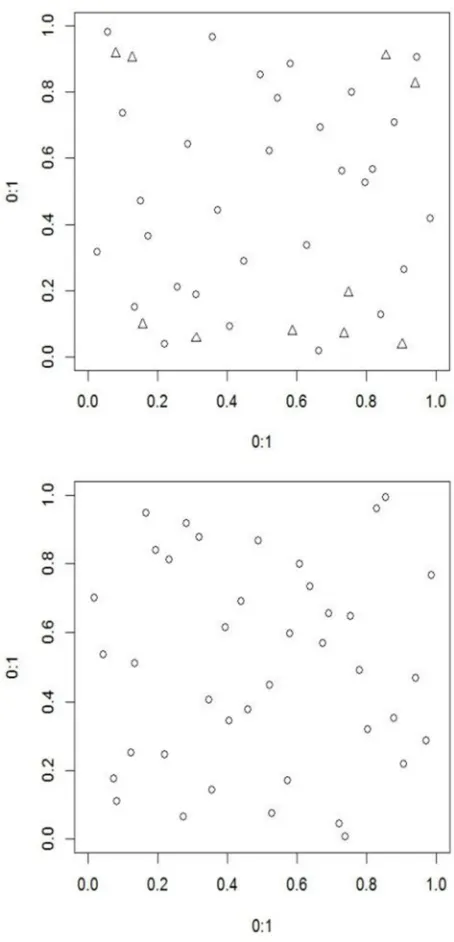
Example 1. Suppose one would like to construct a semi-LHD (40, 2;24). Firstly, an semi-LHD (24, 2), denoted by D₁ is generated as the built-in LHD. Next, eight marginal points are found from D₁. Following the steps of Algorithm 1, two extra points are added to each of the marginal points. Combine all the added points with points in D₁ to obtain the destined design which is denoted by D(1). Similarly, a semi-LHD (40, 2; 30) is constructed which is denoted by D(2). To show the difference between semi-LHDs and LHDs, an LHD (40, 2), denoted by D(3) , is constructed. The bivariate projections for D(1), D(2) and D(3) are visualized in Figure 1. It is not difficult to observe that D(1) has more points near to the edge than D(2) since the built-in LHD of D(1) has less samples than that of D(2) while the sample sizes of D(1)and

(2)

Figure 1. Bivariate projetions for _D(1) (panel on the left), _D(2)(panel in the middle) and _D(3) (panel on the right). Triangles represent the points in semi-LHDs apart from the built-in LHDs.

It worthwhile to note that Steps 1-4 of Algorithm 1 may suffer from an endless loop since the condition a≥a0/ 3 in Step 4 of Algorithm 1 may be hard to achieve. It is thus recommended that the number of circulation should be preset.

3.2. Simulation Studies

Two simulative examples are given in this section to illustrate the usefulness of the proposed design. The prediction performances between random LHDs and semi-LHDs are compared. As for the criteria assessing the prediction performance, the leave-one-out cross-validation error (CVE) and the empirical mean squared prediction error

(MSPE) are adopted. Suppose D=( ,...,x₁ x_n) ' is an n-run design and y*=( ,...,y1 yn) ' is the corresponding response

vector, CVE is then defined as

ɵ 2

1

[ ( ) ( )] , i

i

i i

x x D

CVE y x y x

n _∈ −

=

_∑

− (10)

where ɵ

i x

y₋ is the predicted value of y based on data

\ { }_i

D x and y*\{ }y_i . The definition of MSPE is given by

ɵ 2 1

1

[ ( ) ( )] , N

k k

k

MSPE y x y x N ₌

=

_∑

− (11)

where x₁,...,x_N are testing points selected from the design region. In the simulation, model (2) is established by setting

( ) 1

f x = and β µ= and the parameters are estimated through the maximum likelihood approach introduced in Section 2.

In the simulative examples, the following steps are carried out to assess the prediction performance.

Step 1. Create two data sets A and B . Let A be the collection of N₁ random points drawn from [0,1]p and B be the collection of N₂ points drawn from the area near the edge of [0,1]p.

Step 2. Let t=1,...,N_r . Given t, this step proceeds as follows:

(1) Construct a semi-LHD (n p n, ; ₀), denoted by X_1t, and conduct the computer experiment based on X_1t to obtain the response vector y_1t . Fit model (2) based on {X_1t,y_1t} . Calculate CVE in (10) and denote the result by c_1t. Calculate MSPE in (11) based on A and B and denote the results by

1t

a and b_1t, respectively.

(2) Construct an LHD ( ,n p), denoted by X_2t , and conduct the computer experiment based on X_2tto obtain the response vector y_2t. Fit model (2) based on {X_2t,y_2t}. Calculate CVE in (10) and denote the result by c2t. Calculate

MSPE in (11) based on A and B and denote the results by

2t

a and b_2t, respectively.

Step 3. Let ( ₁,..., ) ', ( ₁,..., ) '

r r

j j jN j j jN

a = a a b = b b and

1

( ,..., ) ' r

j j jN

c = c c for j=1, 2.

Step 4. Calculate the mean and standard deviation of elements in the vectors obtained in Step 3.

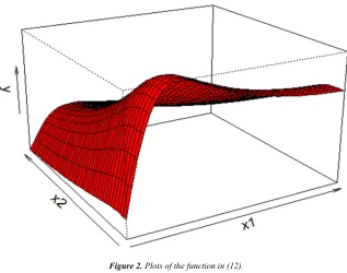
Example 2. Consider a function from Currin, Mitchell, Morris and Ylvisaker (1991) which is given by

3 2

1 1 1

3 2

2 1 1 1

2300 1900 2092 60

1

[1 exp( )] .

2 100 500 4 20

x x x

y

x x x x

+ + +

= − −

+ + + (12)

Once an experimental design is arranged, the response vector can be obtained from Eq.(12). As described at the beginning of this section, two testing data sets A and B are created where the former are collections of 40 points of a random LHD in [0,1]2and the latter 40 points drawn from area near

the edge of [0,1]2. The simulation is repeated 1000 times (i.e., N_r =1000) and and in each time a semi-LHD (30, 2, 20) and an LHD (30, 2) are generated. The prediction performances of the semi- LHD (30, 2, 20) and the LHD (30, 2) are listed in Tables 1 and 2.

From Table 1 it is easy to see that when the testing data set is A, the prediction performance of semi-LHDs compares favorably to that of LHDs. On the other hand, when the

testing data set is B, the mean and standard deviation of MSPE of semi-LHDs are considerably smaller than those of LHDs. This indicates that the proposed designs benefit the prediction capability on the area near to the edge while still behave well over the entire design region. Note that both of these design types have lower prediction accuracies on set B

than set A. This is expected because predicting on the edge of the design region usually has more uncertainty, especially for industrial engineering experiments. Table 2 displays the CVE values from which the advantage of semi-LHDs over LHDs is also obvious.

Example 3. In this example, the following function

1 2 3

log(0.01 ) 10 exp( ) 5 30

y= − +x + x + x (13)

Figure 2. Plots of the function in (12).

Table 1. Means and standard deviations of the MPSE in Example 2, where the number in the parentheses is the standard deviation.

Data set A (LHD) Data set B (edge)

semi-LHD 0.1235(0.1174) 0.1622(0.2726)

LHD 0.1196(0.1378) 0.2721(0.3916)

Table 2. Means and standard deviations of the CVE in Example 2, where the number in the parentheses is the standard deviation.

CVE

Semi-LHD 0.1434(0.1462)

LHD 0.2665(0.3060)

is used as the deterministic computer model. Similar to Example 2, two testing data sets A and B are created where the former are collections of 40 points of a random LHD in

3

[0,1] and the latter 40 points drawn from area near the edge

of [0,1]3. The simulation is repeated 1000 times (i.e., N_r = 1000) and in each time a semi-LHD (30, 3, 20) and an LHD (30, 3) are generated. The prediction performances of the semi-LHD (30, 3, 20) and the LHD (30, 3) are listed in Tables 3 and 4.

Table 3. Means and standard deviations of the MPSE in Example 3, where the number in the parentheses is the standard deviation.

Data set A (LHD) Data set B (edge)

semi-LHD 0.7178(0.6164) 0.8275(1.0019)

LHD 0.6961(0.4032) 1.0059(0.8824)

Table 4. Means and standard deviations of the CVE in Example 3, where the

number in the parentheses is the standard deviation.

CVE

Semi-LHD 0.2149(0.2395)

From Tables 3 and 4, similar conclusions as in Example 2 can be drawn. That is, Semi-LHDs benefit the prediction accuracy on the edge area while still behave well over the entire design region.

4. Conclusion

With the advent of computing technology and numerical methods, industrial engineers frequently use computer simulations to study actual or theoretical physical systems. Typically, the simulation model is resource-intensive in terms of model preparation, computation, and output analysis. As a result, the availability of a “cheap-to-compute” statistical model as a surrogate to the original complex simulation model is particularly useful. To establish a high quality statistical model, choosing a good set of design points is an important issue. In this paper, a novel type of experimental design, namely semi-LHD is proposed and applied to simulation-based industrial engineering experiments. Compared to the most commonly-used Latin hypercube design [8], the proposed design has advantage in helping making predictions on the edge of the design region where the behavior of the response often exhibits substantial uncertainty for an industrial engineering process. An explicit design construction algorithm is given and simulation studies confirm that the proposed semi-LHDs are desirable for computer simulation-based industrial engineering experiments because they can yield good prediction accuracy not only in the interior but also on the edge area of the experimental domain.

Acknowledgements

This work was partially supported by the National Natural Science Foundation of China (Grant No. 11701109).

References

[1] Zhang, Y. and Notz, W. I. (2015). Computer experiments with qualitative and quantitative variables: a review and reexamination. Quality Engineering, 27, 2-13.

[2] Huang, H. Z., Lin, D. K. J., Liu, M. Q. and Yang, J. F. (2016). Computer experiments with both qualitative and quantitative variables. Technometrics 58, 495-507.

[3] Nie, X., Huling, J. and Qian, P. Z. G. (2017). Accelerating large-scale statistical computation with the GOEM algorithm. Technometrics 59, 416-425.

[4] Pareek B., Ghosh, P., Wilson, H. N., Macdonald, E. K. and Baines, P. (2018). Tracking the Impact of Media on Voter Choice in Real Time: A Bayesian Dynamic Joint Model. Journal of the American Statistical Association, https://doi.org/10.1080/01621459.2017.1419134.

[5] Chen, J. K., Chen, RB, Fujii, A., Suda, R. and Wang, W. (2018). Surrogate-assisted tuning for computer experiments with qualitative and quantitative parameters. Statistica Sinica 28, 761-789.

[6] Santner, T. J., Williams, B. J. and Notz, W. I. (2003). The design and analysis of computer experiments. New York: Springer.

[7] Fang, K. T., Li, R. and Sudjianto, A. (2006). Design and modeling for computer experiments.New York: CRC Press. [8] McKay, M. D., Beckman, R. J. and Conover, W. J. (1979). A

comparison of three methods for selecting values of input variables in the analysis of output from a computer code. Technometrics 21, 239-245

[9] Wang, L., Yang, J. F., Lin, D. K. J. and Liu, M. Q. (2015). Nearly orthogonal Latin hypercube designs for many design columns. Statistica Sinica 25, 1599-1612.

[10] Yang, X., Yang, J. F., Lin, D. K. J. and Liu, M. Q. (2016). A new class of nested orthogonal Latin hypercube designs. Statistica Sinica 26, 1249-1267.

[11] Chen, H., Huang, H. Z., Lin, D. K. J. and Liu, M. Q. (2016). Uniform sliced Latin hypercube designs. Applied Stochastic Models in Business and Industry 32, 574-584.

[12] Wang, X. L., Zhao, Y. N., Yang, J. F. and Liu, M. Q. (2017). Construction of (nearly) orthogonal sliced Latin hypercube designs. Statistics and Probability Letters 125, 174-180. [13] Currin, C., Mitchell, T. J., Morris, M. D. and Ylvisaker, D.

(1991). Bayesian prediction of deterministic functions with applications to the design and analysis of computer experiments. Journal of the American Statistical Association 86, 953-963.

[14] Joseph, V. R., Hung, Y. and Sudjianto, A. (2008). Blind kriging: A new method for developing metamodels. ASME Journal of Mechanical Design 130, 031102-1-8.

[15] Kennedy, M. C and O'Hagan, A. (2000). Predicting the output from a complex computer code when fast approximations are available. Biometrika87, 1-13.