A Self-Adaptive Differential Evolution
Algorithm with Dimension Perturb Strategy
Wei-Ping Lee
Information Management Department Chung Yuan Christian University
Chung li, Taiwan [email protected]
Chang-Yu Chiang
Information Management Department Chung Yuan Christian University
Chung li, Taiwan [email protected]
Abstract—Differential Evolution (DE) has been proven to be an efficient and robust algorithm for many real optimization problems. However, it still may converge toward local optimum solutions, need to manually adjust the parameters, and finding the best values for the control parameters is a consuming task. In this paper that proposed a dimension perturb strategy and self-adaptive F value in original DE to increase the exploration ability and exploitation ability. Self-adaptive has been found to be highly beneficial for adjusting control parameters. The performance of self-adaptive differential evolution algorithm with dimension perturb strategy (PSADE) is showed on the following performance measures by benchmark functions: the solution quality and solution stability. This paper has found that PSADE can efficiently find the global value of these functions.
Index Terms—Differential Evolution, Dimension Perturb Strategy, Self-adaptive
I. INTRODUCTION
The differential evolution algorithm (DE) was proposed by Storn and Price in 1996 [12] [14] [15], the algorithm is a popular optimization algorithm in recent years. Previous studies can be found that DE shows better results than other algorithms such as genetic algorithm (GA) and particle swarm optimization (PSO), in addition, DE is used in various fields widely.
Differential evolution is based on random population based global algorithm, like other evolutionary algorithm framework. It is not only well-known, robust, easy to use, fast convergence, but also requiring relatively little control parameters in solving optimization problems. Although DE has the advantages mentioned above, it encounters the crucial flaws of evolutionary computation, like trapped in the local solution easily, and adjust the parameters manually [12] [17].
In the past studies, the differential algorithm had much in common the improved methods that has improve control parameters [1] [4] [7] [16], modify the algorithm framework for process [3] [11] and with other algorithms [9] [17], the main purpose of these methods are trying to
improve exploration ability and exploitation ability. Exploration means that the search to the global optimum capacity in the solution space, when the exploration capability is poor, the algorithm is easily trapped in the local optimum. And the exploitation ability means in the vicinity of global optimum solution can dig out the better solutions, if without adequate exploitation capacity that will cause instability in convergence, stretching computation time and lowering the quality of the solution.
Furthermore, the user must find the best parameter values for different problems. Finding the best values for the control parameters is a time consuming task [17].
Therefore, this paper presented a modified the control parameter and dimension perturb strategy. Through the above mentioned ways to improve
DE has to manually adjust the parameters and the optimal solution trapped into the local optimum issues. Followed by high-dimensional experiment to prove the modified algorithm can achieve a balance between the exploration ability and the exploitation ability.
The following of this paper is organized as follows: this paper briefly introduce the original DE algorithm in section II. Section III, A self-adaptive differential evolution algorithm with dimension perturb strategy (PSADE) is presented in detail. In section IV, the experimental settings and the experiment results are reported the PSADE performed on the benchmark functions. And this paper elaborates the findings in final section.
II. LITERATURE REVIEW
A. Evolution Computation
evolutionary algorithm, is for solving many NP-hard optimization problems in engineering and science related fields [8].
Evolutionary algorithms (EAs) are population-based search algorithms to simulate the evolution of individual select, mutate and recombine process. According to the concept of evolutionary algorithm, the developed specifications include the following steps [8]:
The initial phase: the initial population randomly generated.
Assessment phase: assessment fitness for each individual of population. If meet the termination conditions will be terminated. Otherwise, continue the following steps.
The selection phase: first, the individual selected from the group as a parent. Second, the parent through the various genetic operators to produce new offspring. Finally, assess the fitness value of offspring.
Production phase: the decision to replace some or entire individual of the current group to become the next generation and then back to assessment phase.
B. Differential Evolution Algorithm
Differential evolution is a floating-point encoding of evolutionary algorithms for continuous global optimization solution space, it also can be discrete coding manner [2] [7] [10]. Differential evolution algorithm is similar to genetic algorithm used by the individuals composed of population to search for the optimal solution. But the biggest difference between genetic algorithm and differential algorithm is the mutation operators. Genetic algorithm only use small probability to implement the mutation operator.
On the other hand, mutation in the DE is the use of arithmetic formula to combine the individual in each generation. The mutation plays the role of explores at the beginning and becomes a developer at later evolution process, its individuals within their group will become increasingly similar [6] [12].
The original DE is introduced in more detail with reference to three main operators: mutation, recombination and selection [13] [14] [15].
Mutation
For each individual vector,xi(t), of generation t, a mutant vector is created by
)) ( ) ( ( ) ( )
(t x1 t F x2 t x3 t
vi = r + r − r (1)
where xr1(t), xr2(t) and xr3(t)are randomly selected with i≠r1≠r2≠r3 , and the F is scale factor used to effect the amplification of the difference vector, xr2−xr3 ,
] 2 , 0 [ ∈
F .
Recombination
DE adds the diversity of population that uses a discrete recombination way where elements from the target vector, xi(t) , are combined with elements from the mutant vector,vi(t), to produce the trial vector,ui(t).
⎪⎩ ⎪ ⎨
⎧ < =
=
otherwise t
x
r j or CR rand if t v t u
ij ij
ij ()
) ( )
( (2)
where j=1,…,Nd refers to a specific dimension, Nd is the number of parameters of single individual, and
rand~U(0,1), in the above, CR is the probability of crossover, CR∈[0,1] , and r is the randomly selected index, r~U(1,…,Nd). In other words, the trial vector inherits directly some of elements of the mutant vector, Thus, even CR=0, at least one of the elements of the trail vector randomly selected.
Selection
To select the trial vectorui(t)or target vectorxi(t), DE employs a very easy selection process. Only when the fitness of the trial vector is better than the target vector that the generated trial vectorui(t) replaces the target vector xi(t)be a member of the next generation. For example, if this paper has the same functions in this paper for a minimization problem, the following selections rule such as:
⎩ ⎨
⎧ <
= +
else t x
t x f t u f t u t
x
i
i i
i
i (),
)) ( ( )) ( ( ), ( ) 1
( (3)
where if the trial vector has smaller or equal fitness value than the corresponding target vector, the trial vector will replace the vector, otherwise, the target vector still remain in the population.
Recently, self-adaptive has been proven to be very useful in the automatic and dynamic adjustment of the evolution algorithm of control parameters such as mutation rate and crossover rate. Self-adaptive evolution strategy allows re-configuration to adapt to any general problems [2].
In DE, self-adaptive often used in mutation and recombination of the control parameters, the differential evolution algorithm to set the control parameters mutation and recombination than the third set control parameters on number of population is more sensitive [2].
Sum up, we can be divided into two main types of setting parameter values; parameter tuning and parameter control, parameter tuning is a more common approach is to find out the true meaning of the parameter values before the implementation of the algorithm, and then adjustment algorithm using these values. The parameter control is the parameter value during generation will change and this change can be divided into three [2][5]. Deterministic parameter control:
It’s changed with a number of decisive rules for parameter value.
Adaptive parameter control:
Parameter value assignment strategy may involve some form of feedback mechanism used to determine the direction of the search with (or) significant changes in policy parameters.
Self-adaptive parameter control:
better indivi survive and p
Figu
III. A S A
In this sec of differentia strategy. Th individuals individuals t Hence, the D and to contin
In additio DE/rand/1 s adaptive in F
rate in sol scholars wan the impleme many experi the best s experiment i the concept individual of A. Dimen First, the c carry out the selected to p action from t is that at differences o mechanism c to global exp the differenc Spher Schwef problem Step Setting
iduals. In oth produce offspr
ure 1. Types o
SELF-ADAPTIV ALGORITHM W
STRA ction, this rese
al algorithm his research
trap into the the opportunit DE can increa nue the evoluti on, this study trategy of di
F, F values a ving differen nt to manually entation proce ments can be setting param is a very tim
is to retain f the next stag nsion Perturb S
current iterati e action dimen perform the ex the best indiv the beginnin of each individ can be achiev ploration. The ces between re fel’s 2.22 p Tunin Cont
her words, it ring.
of setting param
VE DIFFERENTI WITH DIMENSIO
ATEGY(PSAD earch will imp and import d anticipates e local optim ty to escape th ase the divers ion in the sam y take the m ifferential alg are about with
nt optimizati y adjust to the ess, they will e found. In oth
meter value me-consuming
n good F va e as a referenc Strategy
on of the best nsion perturb, xchange of tw vidual vector. ng of evolut dual vector is ved through th en in the latter
individual ve
Benchmark f
f1
= x f2( )
=
x f3( ) ng
rol
D
S
will be easi
meters [5]
IAL EVOLUTIO ON PERTURB DE)
prove the stru dimension pe
that when mum, it can
he local optim sity of popula me time.
most widely gorithm with h the converg ion problems e best paramet l have to by her words, fin from diff work. There alues and let ce.
t individual v , that is, rand wo elements o Its main obje tion, due to very large, su he jumping ab r part of evolu ectors will sl
Table I. functions
∑
= = n i x x 1 ) (∏
∑
= + = n i i x 1⎣
(
∑
= + = n i i x 1 Deterministic Adaptive Self-adaptive er to ON ucture erturb the give mum. ation, used self-gence s. If ter in very nding ferent efore, t the vector omly of the ective o the uch a bility ution, lowly shrin enha from B. Th and The indiv Th with begi this curr ) (t vi whe (t Fi Th gene unde gene succ a sp for s mea vect mec reco and proc durin prop learn In unim cont type solu and Benchmark f i x2∏
= n i i x 1⎦
)
2 5 . 0nk, and then ance the popu m the local opt
F value of S he F value is
different test concept is vidual of the n his study assu h mean Fa
inning, Fa is s normal distr ent population
( ) ( )=xr1t +Fi
ere 15 . 0 , ( ) N Fa t =
hese F value erations and t er the same eration, the F
cessfully enter pecified numb several times an Fa and stan
tor to be s hanism to th orded along. W the standard cess. In additio
ng this period per F value r
ned to suit thi
IV n this study, t modal as wel
tains small an es, the assessm ution to the me
stability of pe
functions fmi
0
0
0
n through the ulation diversit
timum. Self-adaptive
related to the functions may to retain go next stage as a umes F norm and standard set at 0.5 and ribution are f n. The method
) ( ( * )
(t xr2 t −x
) 5
s for all indiv then a new se e normal di
F values ass ring the next g ber of generat
under the sam ndard deviation successful re he next gene With this new
d deviation 0 on, if there ar d, the Fa will n
range for the s problem.
V. EXPERIME the test functi ll as the mu nd large local
ment criteria ean and stand erformance as
n S
[-100,10
[-10,10
[-100,10
e perturb me ty and the abi
solution conv y have the bes od F values a reference. mally distribut
d deviation different F va for each indiv d is then calcu
)) ( 3 t
xr
viduals remai et of F values istribution. D ociated with generation are tions, F has b me normal dist n 0.15, and af eservations v
eration, F v normal distrib .15, we repe re no successfu
not change. A e current pro
ENT RESULT on can be div ultimodal func l optimum of
will be used dard deviation sessment. Gr 00]D 0]D 00]D echanism can ility to escape
vergence rate, st value itself. and let the
ed in a range 0.15. In the alues conform vidual in the ulated as
(4)
(5) in for several s is generated During every trial vectors e saved. After been changed tribution with fter every trail via selection value will be bution's mean eat the above ful individuals As a result, the oblem can be
vided into the ctions, which f two optimal d to solve the n for precision
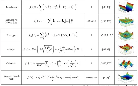
Rosenbrock
∑
(
)
(
)
−
=
− − ⎟⎠⎞
⎜ ⎝
⎛ − + −
= 1
1
2 1 2 2
1
4( ) 100 1
n
i
i i
i x x
x x
f 0 [-30,30]D
Schwefel ‘s
Prblem 2.26
∑
(
( )
)
= −
= n
i
i
i x
x x
f
1
5( ) sin -12569.5 [-500,500]D
Rastrigin
∑
(
(
)
)
=
+ −
= n
i
i
i x
x x
f
1 2
6( ) 10cos 2π 10 0 [-5.12,5.12]D
Ackley’s x e
D x
D x
f
D i
i D
i
i ⎟⎟+ +
⎠ ⎞ ⎜
⎜ ⎝ ⎛ − ⎟⎟ ⎟ ⎠ ⎞
⎜⎜ ⎜ ⎝ ⎛ − −
=
∑
∑
= =
20 ) 2 cos( 1 exp 1
2 . 0 exp 20 ) (
1 1
2
7 π 0 [-32,32]D
Griewank cos 1
4000 1 ) (
1 1
2
8 ⎟⎟ +
⎠ ⎞ ⎜⎜ ⎝ ⎛ −
=
∑
∏
= =
n
i
i n
i i
i x x
x
f 0 [-600,600]D
Six-hump
Camel-back 9 12 14 3 16 1 2 4 22 4 24
1 1 . 2 4 )
(x x x x xx x x
f = − + + − + -1.0316285 [-5,5]D
A. Experiment with Original Differential Evolution
Table II. Experiment parameters setting with original differential evolution
NP 50 Dimension 30
F 0.5
CR PSADE1~N(0.5,0.1) 0.9;
Initial Fa 0.5
Update Fa Generation 50
Generation 1000
This section will be conducted comparison experiment with DE/rand/1, DE/best/2 and DE / current to best / 1. The CR 0.9 of PSADE refer to Storn with Price, and the PSADE1 refer to Qin and Huang, who made use of the normal distribution of mean 0.5 and standard deviation 0.1 for differential individuals in the current population [11]. Other parameters set as shown in table II.
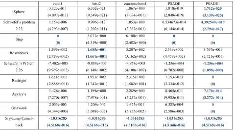
Table V summarizes the results obtained by applying the different methods to the unimodal problems. The result shows that PSADE and PSADE1 performed better than (or at least equal to) the other strategies in all the benchmark functions except the Rosenbrock function where DE/best/2 outperformed the other strategies. However, PSADE1 performed significantly better than PSADE.
Table V summarizes the results obtained by applying the different methods to the multimodal problems. The result shows that PSADE1 performed consistently better than the other strategies in all the test functions. The improvement is even more significant for the Rastrigin
function. Furthermore, examining the standard deviations of all the algorithms, PSADE1 achieved the smallest standard deviation, illustrating that PSADE and PSADE1 are more stable and thus more robust than the other versions of DE.
Fig. 2 shows average best fitness curves for the different strategies with 30 independent runs for selected benchmark functions. Fig. 2 shows that PSADE1 has a faster convergence rate than DE/rand/1, DE/best/2, DE/Current to best/1 and PSADE. On the other hand, the figure shows that PSADE1 converges insignificantly faster than DE/best/2. Hence, from table V and Fig. 2 it can be concluded that, PSADE1 reached the global optimum solution faster than the other strategies in all functions except for the Rosenbrock function.
B. Solution of the effectiveness of Fa update frequency
This section will examine the updated Fa effectiveness. To find out the self-adaptive update frequency will affect or not affect the performance of the solution.
Set of experimental parameters such as table III.
Table III. Experiment parameters setting withupdate Fa
frequency
NP 50 Dimension 30
F 0.5
CR PSADE1~N(0.5,0.1) 0.9;
Initial Fa 0.5
Update Fa Generation 25;50;100
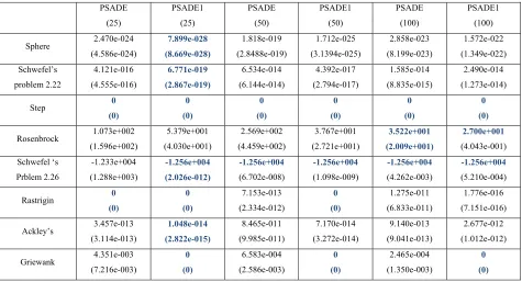
PSADE1 can offer the best output by updating the Fa
value strategy with every 25 iterations, on the other hand, PSADE1 advantage with every 100 iterations to update the Fa value strategies offer more prominent effect output in Rosenbrock function.
Solving multi-modal functions, can still be observed PSADE1 with updates every 25 iteration strategy Fa
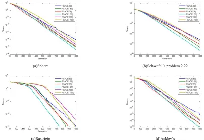
values are output to provide better accuracy and stability. Fig. 3 shows average best fitness curves for the different strategies with 30 independent runs for selected benchmark multimodal functions. Fig. 3 shows that PSADE1 (25) and PASDE1 (50) achieved faster convergence rates than others. Besides, PSADE1 (25) converged insignificantly faster than PSADE1 (50).
Table VI shows the dynamic CR values strategy is better than fix CR values strategy. And different updating strategy of Fa frequency will also affect the accuracy and stability of the solution. Whether in the unimodal or multimodal of the benchmark functions, the updating the
Fa value strategy with every 25 iterations provided the most outstanding results.
C. With BBDE in high-dimension experiment
Table IV. Experiment parameters Setting with BBDE[10] NP 50 Dimension 100
F 0.5
CR PSADE1~N(0.5,0.1) 0.9;
Initial Fa 0.5
Update Fa Generation 25
NFEs 50000
In this section, the function dimension raised to 100. This paper will choose the Omran et al, who published BBDE [10] algorithm to compare the object in 2009. The article has put forward an improved mechanism and control parameters. The BBDE is based on self-adaptive differential algorithm with almost free parameter fine-tuning of the hybrid differential improvement algorithm.
The main motivation is that when encountering new problems, PSO and DE are required to optimize the control parameters set, it can be regarded as the best set parameters dependence. In addition, self-adaptive differential algorithm have been studied to show good solution results, and it can reduce the time that to find the best parameter value of each problems. Therefore, this study will compare this research, to verify the method of this study and conduct precision on the performance comparison.
Set of experimental parameters in table IV. The four of the unimodal functions, the BBDE and PSADE1 presented results superior to the traditional differential algorithm. Hence, comparison results can be seen that BBDE and PSADE1 has the advantage to solve Sphere and Schwefel’s problem 2.22 through the data.
The Step function is not a continuous problem type of the unimodal function, PSADE and PSADE1 still can maintain the effectiveness of the stability of its solution.
But for the Rosenbrock function, BBDE are more prominent than other algorithms. According to unimodal functions of experimental data, PSADE1 and BBDE have faster convergence, more stable and more accurate than the traditional differential algorithm.
For the multimodal functions, the Rastrigin function and Griewank function has a lot of local optimum solutions. Table VII can be found that the PSADE1 has better accuracy than BBDE and traditional differential algorithm. On the other hand, BBDE and the traditional differential algorithm are not particularly outstanding to solve these functions.
For the Ackley function, BBDE and PSADE1 are able to meet the better stability and accuracy. Therefore, in multimodal test functions, PSADE1 algorithm presented the excellent results in the same condition. In other words, when PSADE1 encounter more complex and more local optimum solution multimodal functions, the application of perturb strategy have the opportunity to escape from the region and self-adaptive of F values can fast convergence in every function.
V. CONCLUSION
The differential algorithm through the self-adaptive parameter F and the dimension perturb strategy is to make up for the shortcomings. In order to enhance the exploration ability, exploitation ability and increase the population diversity, so that algorithms can be more appropriate speed convergence towards the optimal solution and effectively promote to escape from the local optimum.
Expectations effectively enhance the effectiveness of the algorithm for solving accuracy and stability. Meanwhile, the conclusions are sorted out from the experiment.
First, the parameters tuning is a time-consuming work, therefore, this study use self-adaptive mechanism for F
value, it can reduce the need for different functions to do manually adjust the parameters to find the best setting time. Second, when trapped into the local optimum, the algorithm with dimension perturb strategy can enhance the capacity of the escaping from local optimum area. Third, if the problem complexity increases, the PSADE1 is able to maintain a stable and accurate status for solving effectiveness. Finally, the convergence evolution diagram can understand that the proposed algorithm has fast convergence speed. In other words, PSADE1 can be reached with less iteration to evolution.
REFERENCES
[1] Abbass, H.A. The self-adaptive Pareto differential evolution algorithm. in Evolutionary Computation, 2002. CEC '02. Proceedings of the 2002 Congress on. 2002. [2] Brest, J., et al., Performance comparison of self-adaptive
and adaptive differential evolution algorithms. Soft Computing - A Fusion of Foundations, Methodologies and Applications, 2007. 11(7): p. 617-629.
Intelligent Systems and Applications, 2009. ISA 2009. International Workshop on. 2009.
[4] Das, S., A. Konar, and U.K. Chakraborty. Improved differential evolution algorithms for handling noisy optimization problems. in Evolutionary Computation, 2005. The 2005 IEEE Congress on. 2005.
[5] Eiben, A.E., R. Hinterding, and Z. Michalewicz, Parameter control in evolutionary algorithms. Evolutionary Computation, IEEE Transactions on, 1999. 3(2): p. 124-141.
[6] Gong, W., Z. Cai, and L. Jiang, Enhancing the performance of differential evolution using orthogonal design method. Applied Mathematics and Computation, 2008. 206(1): p. 56-69.
[7] Junhong, L. and L. Jouni. A fuzzy adaptive differential evolution algorithm. in TENCON '02. Proceedings. 2002 IEEE Region 10 Conference on Computers, Communications, Control and Power Engineering. 2002. [8] Kicinger, R., T. Arciszewski, and K.D. Jong, Evolutionary
computation and structural design: A survey of the state-of-the-art. Computers & Structures, 2005. 83(23-24): p. 1943-1978.
[9] Luitel, B. and G.K. Venayagamoorthy. Differential evolution particle swarm optimization for digital filter design. in Evolutionary Computation, 2008. CEC 2008. (IEEE World Congress on Computational Intelligence). IEEE Congress on. 2008.
[10]Omran, M.G.H., A.P. Engelbrecht, and A. Salman, Bare bones differential evolution. European Journal of Operational Research, 2009. 196(1): p. 128-139.
[11]Qin, A.K., V.L. Huang, and P.N. Suganthan, Differential Evolution Algorithm With Strategy Adaptation for Global Numerical Optimization. Evolutionary Computation, IEEE Transactions on, 2009. 13(2): p. 398-417.
[12]Salman, A., A.P. Engelbrecht, and M.G.H. Omran, Empirical analysis of self-adaptive differential evolution. European Journal of Operational Research, 2007. 183(2): p. 785-804.
[13]Storn, R. On the usage of differential evolution for function optimization. in Fuzzy Information Processing Society, 1996. NAFIPS. 1996 Biennial Conference of the North American. 1996.
[14]Storn, R. and K. Price. Minimizing the real functions of the ICEC'96 contest by differential evolution. in Evolutionary Computation, 1996., Proceedings of IEEE International Conference on. 1996.
[15]Storn, R.,K. Price., Differential Evolution - A simple and efficient adaptive scheme for global optimization over continuous spaces. Technical report, California: International Computer Science Institute, Berkeley., 1995. [16]Das, S., A. Konar, and U.K. Chakraborty. Two improved
differential evolution schemes for faster global search. GECCO '05: Proceedings of the 2005 conference on Genetic and evolutionary computation, 2005.
[17]Zhi-Feng, H., G. Guang-Han, and H. Han. A Particle Swarm Optimization Algorithm with Differential Evolution. in Machine Learning and Cybernetics, 2007 International Conference on. 2007.
Wei-Ping Lee received the the Ph.D. degrees in Institute of Computer Science and Information Engineering from National Chiao Tung University, Hsinchu, Taiwan, R.O.C.
Currently, he has been an Assistant Professor in the Department of at Chung Yuan Christian University Chung li, Taiwan, R.O.C. His research interests include the global optimization, evolutionary algorithms, data mining and AI applications.
Chang-Yu Chiang received the master degree in Information Management from Chung Yuan Christian University, Chung li, Taiwan, R.O.C.
His interests include the global optimization, evolutionary algorithms and data mining.
Table V. Mean and standard deviation (SD) of the optimization results for 30 runs
rand1 best2 currenttobest1 PSADE PSADE1
Sphere 3.123e-011 (4.097e-011)
6.352e-021 (9.549e-021)
1.867e+000 (8.064e-001)
1.818e-019 (2.848e-019)
1.712e-025 (3.139e-025)
Schwefel’s problem 2.22
1.154e-006 (4.293e-007)
9.996e-012 (1.202e-011)
1.053e+000 (2.267e-001)
6.534673e-014 (6.144e-014)
4.392549e-017 (2.794e-017)
Step 0
(0)
3.633e+000 (4.319e+000)
6.100e+000 (2.482e+000)
0 (0)
0 (0)
Rosenbrock 1.299e+002 (2.729e+002)
1.685e+001 (1.661e+001)
3.207e+002 (3.162e+002)
2.569e+002 (4.459e+002)
3.767e+001 (2.721e+001) Schwefel ‘s Prblem
2.26
-7.402e+003 (9.969e+002)
-9.888e+003 (6.148e+002)
-4.958e+003 (4.100e+002)
-1.256e+004
(6.702e-008)
-1.256e+004 (1.098e-009)
Rastrigin 1.631e+002 (2.888e+001)
1.951e+002 (1.743e+001)
2.315e+002 (1.582e+001)
7.153e-013 (2.334e-012)
0 (0)
Ackley’s 1.426e-006 (7.270e-007)
1.199e+000 (7.978e-001)
2.289e+000 (5.257e-001)
8.465e-011 (9.985e-011)
7.170e-014 (3.272e-014)
Griewank 2.053e-003 (4.344e-003)
1.206e-002 (1.088e-002)
9.675e-001 (5.725e-002)
6.583e-004 (2.586e-003)
0 (0)
Six-hump Camel-back
-1.0316285 (4.5168e-016)
-1.0316285 (4.5168e-016)
-1.0316285 (4.5168e-016)
-1.0316285 (4.5168e-016)
(a)Sphere (b)Schwefel’s problem 2.22
(c)Rastrigin (d)Ackley’s
Figure 2. Convergence Graph for the optimum solution
Table VI. Mean and standard deviation (SD) of the optimization results for 30 runs PSADE
(25)
PSADE1 (25)
PSADE (50)
PSADE1 (50)
PSADE (100)
PSADE1 (100)
Sphere 2.470e-024 (4.586e-024)
7.899e-028 (8.669e-028)
1.818e-019 (2.8488e-019)
1.712e-025 (3.1394e-025)
2.858e-023 (8.199e-023)
1.572e-022 (1.349e-022) Schwefel’s
problem 2.22
4.121e-016 (4.555e-016)
6.771e-019 (2.867e-019)
6.534e-014 (6.144e-014)
4.392e-017 (2.794e-017)
1.585e-014 (8.835e-015)
2.490e-014 (1.273e-014)
Step 0
(0)
0 (0)
0 (0)
0 (0)
0 (0)
0 (0)
Rosenbrock 1.073e+002 (1.596e+002)
5.379e+001 (4.030e+001)
2.569e+002 (4.459e+002)
3.767e+001 (2.721e+001)
3.522e+001 (2.009e+001)
2.700e+001
(4.043e-001)
Schwefel ‘s Prblem 2.26
-1.233e+004 (1.288e+003)
-1.256e+004 (2.026e-012)
-1.256e+004
(6.702e-008)
-1.256e+004
(1.098e-009)
-1.256e+004
(4.262e-003)
-1.256e+004
(5.210e-004)
Rastrigin 0
(0)
0 (0)
7.153e-013 (2.334e-012)
0 (0)
1.275e-011 (6.833e-011)
1.776e-016 (7.151e-016)
Ackley’s 3.457e-013 (3.114e-013)
1.048e-014 (2.822e-015)
8.465e-011 (9.985e-011)
7.170e-014 (3.272e-014)
9.140e-013 (9.041e-013)
2.677e-012 (1.012e-012)
Griewank 4.351e-003 (7.216e-003)
0 (0)
6.583e-004 (2.586e-003)
0 (0)
2.465e-004 (1.350e-003)
(a)Sphere (b)Schwefel’s problem 2.22
(c)Rastrigin (d)Ackley’s
Figure 3. Convergence Graph for the optimum solution
Table VII. Mean and standard deviation (SD) of the optimization results for 30 runs
rand1 best2 BBDE[10] PSADE PSADE1
Sphere (40.145155) 32.091642 (2.750338) 1.959712 (0.000000) 0.000000 (0.000045) 0.000046 (0.000000) 0.000000 Schwefel’s
problem 2.22
1.544770 (1.189442)
0.760741 (0.671501)
0.000000 (0.000000)
0.000151 (0.000071)
0.000000 (0.000000)
Step (220.6941) 158.8333 (522.7707) 932.7 (5.01824) 2.70000 (0.000000)0.000000 (0.000000)0.000000
Rosenbrock (168799.9) 85618.17 (93453.1) 72253.2 (195.54631)312.63207 (525.9118) 835.0324 (475.7651) 562.1907
Rastrigin (71.39962) 774.7837 (232.3332) 806.7959 616.194754 (38.11584) (3.239625) 1.292809 (0.001623)0.001120
Ackley’s (0.472041) 2.435670 (1.129922) 6.881239 (0.000001)0.000000 (0.000187) 0.000528 (0.000001) 0.000004
![Table IV. Experiment parameters Setting with BBDE[10]](https://thumb-us.123doks.com/thumbv2/123dok_us/7832107.1667313/5.595.66.284.361.472/table-iv-experiment-parameters-setting-with-bbde.webp)