Prediction Algorithm for State Prediction Model

(1)

Prediction Algorithm for State Prediction Model

Zili Zhang

Computer Science Department, Shijiazhuang University, Shijiazhuang, China [email protected]

Hongwei Song

Computer Science Department, Shijiazhuang College, Shijiazhuang, China [email protected]

Yan Li

Computer Engineering Department, Ordnance EngineeringCollege,Shijiazhuang, China Hao Yang

Computer Science Department, Nanjing Normal University, Nanjing, China

Abstract—Dynamic Bayesian network is the extension of Bayesian network in solving time series problems .It can be well dealt with the time-varying multivariable problem. A state model is given based on Dynamic Bayesian network. The model can more accurately describe the relationship between the system state and the influencing factors. Single-step and multi-step prediction algorithms are given to predict the system state. The multi-step state prediction algorithm is achieved by extending time-slice. In this paper, the width of the reasoning is used to simplify the amount of data in the reasoning process.

Index Terms – dynamic Bayesian networks, state prediction model, single-step prediction algorithm, multi-step prediction algorithm

Ⅰ. INTRODUCTION

Bayesian networks, also known as belief networks, are already well-established as representations of domains involving uncertain relations among several random variables. Dynamic Bayesian network, the extension of Bayesian network in solving time series problems and the reducible model for complex random progress, which variables evolve with time, can effectively represent and solve the multi-variables’ problem [1,2]. Dynamic Bayesian Networks (DBNs) have been receiving increased attention as a tool for modeling complex stochastic processes, especially that they generalize the popular Hidden Markov Models (HMMs) and Kalman lters. In time series modeling, we observe the values of certain variables at different points in time. The assumption that an event can cause another event in the future.

It is very important for makers to predict the state of system. But the state prediction is very difficult because the state of the system is generally affected by many random factors. The random variable can evolve with time in dynamic Bayesian network. The DBNs have also been widely used to reason and predict[3]_{. A dynamic}

system can be represented by a state-space model. The state prediction model based on DBNs is mainly used to solve the state prediction for the system affected by many random factors. A single-step prediction algorithm is proposed to adjust time forecast. However, the prediction

is difficult to the case that the forecast time is far away from the current time. This paper proposes a multi-step prediction algorithm which can be used to solve this problem.

We begin with formal description of the state prediction model. In the section, we proposed two algorithms to respectively determine factors and dependences. Section 3 discusses the support degree among all nodes and variable transition probabilities of nodes. We propose forward and backward algorithms in the end of this section. In section 4, this paper proposes a definition of interface span to greatly reduce data storage space. In Section 5, this paper gives the single-step prediction algorithm and the multi-step prediction algorithm. Section 6 finally ends with an experiment.

Ⅱ. STATE PREDICTION MODEL

Our task is to predict thestate of a system for making a reasonable decision. Recently, there has been a surge of interests along this direction[4,5,6,7]. Firstly, we give a model for state prediction based on Dynamic Bayesian networks. Dynamic Bayesian networks are a class of Bayesian networks specifically tailored to model temporal consistency present in some data sets. In addition to describing dependencies among different static variables, DBNs[8]_{describe probabilistic}

dependencies among variables at different time instance. A set of random variables at each time instance t is represented as a static BN. A major benefit of the DBNs is that their well-constrained network structure allows for simplified inference. Therefore we give a state prediction model based on Dynamic Bayesian networks.

A. A summary of Model Structure

(2)

the state node within a slice. We assume that these dependencies between nodes at neighboring time slice satisfy the Markov assumption [9]._{.The kind of state}

prediction is illustrated as follows:

With the topology shown in Figure 3.1, we firstly give necessary instructions of some symbols in the prediction model to the description and use in lower sections.

State space is expressed as Q={ ,q q₁ ₂…qn}.So we

can use Q_t to express the state at time t, and q_t∈Q

denotes the arbitrary value of the state. Assigning a time index t to each variable, the symbol {Q Q₁, ₂…QT} is a

sequence of state. This paper assumes that T_i is the average of the sampling interval of all state nodes in Q.

Assigning a number index i to each variable, the vector

V

=

{ ,

V V

₁ ₂

…

V

_m

}

expresses m influence factors. The ith influence factor will be denoted by Vi and its

space of values expressed by

V

_i

=

{

v v

_i₁

,

_i₂

…

v

_ik

}

.Let

t

V describe the vector of an influence factor at time

t

.So the ith variable could be denoted by t i

V

and its exact value is t

ij

v

.

With the help of symbols described above, the state predication model can be represented with the sate sequence

0:T

Q and a vector sequence of factors

V

_0:_T.

There are two conditional independence relations among all nodes and these relations could be respectively described by I( ,V_t {Q_{0: 1}_t₋ ,V_{0: 2}_t₋ } |V_t₋₁) and

} | { 0: 1 0: 1

{ , ₁

( ,Q_t Q _t V _t Q , })V

t t

I ₋ ₋ ₋ .

So, from basic probability theory we know that we can factor the join probability as a product of conditional probabilities in the model:

0 : 0 : )

(

T T

p Q V =

0) ( 0 0)

( p

|

p V Q V .

1 1

( |_t _t ) ( _t| _t _t) t

p V V ₋ p Q Q ₋ V

∏

B. The selection of influence factors

Firstly, we should construct the state prediction model. The knowledge of basically framework of the model known from the expert makes it important to determine all influence factors and the dependent relationships

between them at the adjacent time slices. The result of selection factors will directly affect the state prediction. According to the actual situation, factors should meet two basic requirements: effectiveness and non-redundancy. The so-called effectiveness is that factors can play a role to the state. The validity of factors could be tested by the average mutual information I Q V( ; )i between the

influence node and the statute node. If I Q V( ; )_i >τ (

τ

is a given threshold value), then we believe that the factor meets effectiveness. The so-called non-redundancy is that there is less mutual information between the factors at the same time. The non-redundant can be detected by the average mutual information between the factorsI( ; )V V_i _j .

If I( ; )V V_i _j <ξ (

ξ

is a given threshold), then it is

considered that

i

V and V_j meet the non-redundancy. Let U be a set of the candidate factors, Vbe the selection set of the influence factors. Then the selection algorithm of influential factors is such as algorithm 3.1.

Algorithm 3.1. Set V = ∅,_V'_{= ∅}

For

i

=1 to

| |

U

If _{( ; )}

i

Q U

I >

τ

then add Ujto

V

' Sort '

i

V into an order decreasing by I Q V( ; )_i'

For

j

=1 to _| '_| V

For each V ∈V If _{( ; )}_V' _V

j

I <ξ then add '

j

V to

V

C. Determination of dependency

In this model, the dependence between the state node and factors is obvious, thus it dose not need to learn. According to the selection algorithm of influencing factors, we could obtain that different factors at the same time are mutually independent. Therefore it is only needed to determine dependencies between factors at the adjacent time in this model. The specific algorithm is shown as algorithm 3.2.

Algorithm 3.2 Input t−1₌

V V ,Vt =V For each t 1

j

V

−

∈

V

t−1 For each t

i

V

∈

V

t If

_{( ;}

t t 1

₎

i j

I V V

−

>

ω

then

V

jt−1

→

V

it

Through the choice of factors and dependencies of the selection, the state prediction model of the structure can be determined. We can get the conditional probability table by the statistics of historical data.

D. Two factors

Because we use maximum likelihood estimation to study the state transition probability, we do not consider its variability. The node transition probability calculated by maximum likelihood estimation is an average value and it is time-invariant. The context is different, and although the state node's parent has the same value as these nodes at other times, the state node’s value may be

t-1 t t+1

V

1

1 −

−

=

t

q

Q

t

=

q

t

Q

t+1

=

q

t+1

(3)

different. The context mentioned here refers to the values of influence nodes at the time slice which has two times slice distance with the observation time, thus transition probability of the state node is not always invariant, but has certain variability. This paper introduces two factors: the maintenance factor and transfer factor. Therefore the model can not only handle these time-invariant systems but also deal with these variable systems.

From context, we give judging method to determine whether to consider the changes in the state transition probability at time t. If p q q( | , )i iVt ≥p q q( | ,i iVt−₁), then

changes need to be considered. However, if

1

( | , )

i iVt

( | , )

i i Vt

p q q

<

p q q

₋ , then changes need to be considered.

The possibility of changes in the state transition probability will due to the state duration time and the longer the duration the greater the possibility to change. To solve this problem, this paper constructs two factors: the maintenance factor and transfer factor. These two factors should meet some requirements.

(1) Maintenance factor is in inverse proportion to the duration of the same state. Transfer factor is in inverse proportion to the duration of the same state.

(2)If t is less than or equal to

2 i

T _{, the maintenance} should be more than the transfer factor. If t is larger than

2 i

T _{, the maintenance should be less than the transfer} factor.

Let q_ibe the state value at the current time and T_ithe

average of duration. Assuming that the value of state has a duration t. If the maintenance factor is

γ

and the

transfer factor is _λ, we have

t

i

T

γ α= , i

T t

T i

λ α

−

= .

Where

α

is undetermined coefficient

satisfying0<α≤1. If

α

is equal to one, it shows that the state transition probability meets invariance.

E. Calculation of variable transition probability

Assuming that q

iis the value of the state node at time t. The values of all influence factors are known at time t+1, and they meet p q q( | , )i iVt+₁ <p q q( | , )i iVt .The

state transition probability obtained by maximum likelihood estimates is denoted by '

k

p（k=1, 2,…,n）. The maintenance factor

γ

and transfer factor

_λ

has been known at current time. The state transition probability at time t+1 could be calculated as follows: state

i

q transition probability ispi =ωγ pi' and other

state transition probability is '

j j

p =

ωλ

p . Where

ω

is

the normalization constant and the value is

' '

1

(1 )

i i

p p

ω

γ λ

=

+ −

The value of the variable α should make the formula

'

1

| |

T

t t

t

q q

=

−

∑

to obtain the minimum, where qtis the

predict of the state, '

t

q is the actual value for the state and T is the sampling duration.

Ⅲ THE FORWARD-BACKWARD ALGORITHM

The mentioned evidences refer to all the random variables known values. When you get values of some nodes at predict time slice, you can update the predicted results of nodes unknown value by the support degree among nods. The forward algorithm is that the predicted likelihood of the state node will be updated by the support degree of the influence factors to it. The backward algorithm is that the predicted likelihood of the factor node will be updated by the support degree of the state node to it.

A. Support Degree

There are different influences between events, thus a method is proposed to measure the degree of influence between nodes in paper [10,11]. The results of this method cannot reflect the negative impact between random events. However, the fact is not the case. This article gives a new method to compute the support according to the mutual information between random events. Mutual information between random events

i

x

and

y

_jis as follow:

( |

)

( ;

)

( )

( |

)

log

( )

i j

i j i i j

i

p x

y

I x y

I x

y

p x

=

−

=

If P(xi|yi) is greater than P(xi) ,then I(xi;yi) is larger

than zero. If P(xi|yi) is less than P(xi) ,then I(xi;yi) is less

than zero. If the event xi and the event yi are mutually

independent , then I(xi;yi) equals zero. We can conclude

that some events would have different effects on the same event. Some promote the event, some hinder it, and others have nothing with the random event.

Based on what are discussed above, this definition is given to compute the support degree of influence factors to the state node

Definition 1 Let

v

_ilbe the lth value of the ith influence

factor. Now assuming that the state value is

q

_jat time slice t, and then the support degree of influence factor to state node is

w

_il

=

I v q

( ; )

_il _j

,

and the range is

( ,

_{−∞ +∞}

)

.

According to the above two methods, we can get support degrees among the different nodes. Then we would update the predicted results by the amended algorithms which will be introduced.

B. The relationship between conditional probabilities and mutual information

Let xi be the value of the random variable, then the

probability of X can be described as P(X= xi).

Considering the endless independent random variables, E1, E2… and En, the values of these random variables

are respectively e1, e2, … and en. Thus we can compute

(4)

1 2

( | , ..., )

i n

p x e e

e

＝

1 2

( , , ..., )

( , ..., )

i n

n

p x e e

e

p e e

e

＝

1 2

( ) ( , ..., | )

( , ..., )

i n i

n

p x p e e

e

x

p e e

e

＝

1

( | )

( )

n

j i i

j j

p e

x

p x

p e

=

∏

According to mutual information I(xi;yi) and conditional probability

p(x

i

|e

1

,e

2

,…,e

n

),

we can have

1 ( ; ) 1 2

( | , ..., )

( )

n i j j

I x e

i n i

p x e e

e

p x e

=

∑

=

This expression reflects the relationship among the prior probability, posterior probability and the mutual information.

Thus we can have the methods to update the prediction results by posterior probability and the mutual information.

C. Amendment to the state node

Let qj be the value of the state Q at t+1 time slice,and

the probability of Q would be described as P(Q= qj).

Assuming that_λ_jis the support of evidences to the state qj.

The selection algorithm shows that the influence nodes are independent of each other at the same time slice. Then according to the relationship between mutual information and the posterior probability, the prediction likelihood could be updated by the following formula.

'

1 1

(

)

j

(

)

t j t j

p Q

₊

=

q

=

α

e p Q

λ ₊

=

q

(

j

=

1,2…

,

n

)

In the above formula,

α

is the Normalization Factor, and it’s value is

' 1

1 1

( ) ]

j

n

t j

j

eλ p Q ₊ q −

= =

∑

D Amendment to the influence factors

Let

v

_ilbe the value of the ith influence factor

V

_i at t+1 time slice, then we would use '₍ t1 ₎

i il

p V+ =v to

describe the probability of t 1 i

V

+ . Assuming that

w

_ilis the support degree of the state

Q

_t₊₁to

v

_il . So the prediction likelihood could be updated by the following formula.

1 ' 1

(

t

)

wil

(

t

)

i il i il

p V

+

=

v

=

β

e p V

+

=

v

(

i

=

1,2 ,

"

m

;

1,2 ,

l

=

"

k

).

In the above formula,

β

is the Normalization Factor,

and its value is ' 1 1

1

[

il

(

)]

k

w t

i il l

e

p V

v

β

+ −

=

∑

=

Ⅳ. INFERENCE SPAN

When modeling a large and complex decision problem involving a sequence of decisions, the past observations and decisions of a decision may involve a large set of

variables. If without any restrictions the nodes in all time slices will be needed to store for reasoning the values of nodes at a time slice. Therefore, when the time span is very large, it requires a lot of storage space. However, in fact, the node values at all time slices are not needed to calculate the probability distribution of nodes at the time slice t, and the reasoning span needs to be determined in

order to reduce the time complexity of reasoning. Let T be the reasoning span. When T is determined, we only keep the values of nodes within the time span T. Thus this greatly reduces storage space.

Definition 2[12] The forward interface of a DBN

with span T is the set variables at time

t

<

T

with children at time

t

+

1

.It is represented as follows:

1

{

t

| ( , )

(

1),

t

}

tmp t

F

= ∈

u

V

u v

∈

E

t

+

v V

∈

+

Definition 3[13] The backward interface of a DBN

with span T is the set variables at time

t

<

T

with parents at time

t

−

1

or having children which have parents at time

t

−

1

. It is represented as follows:

{

|

t t

B

= ∈

v V

( , )

u v

∈

tmp

( )

E

t

or

1

( ) : ( , )

tmp

( ),

}

t

w

ch v

u w

E

t u V

−

∃ ∈

∈

.

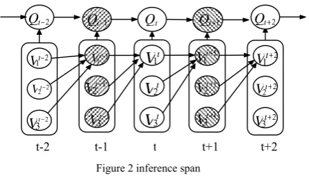
Based on the above two definitions and combining with the characteristics of the prediction model, this paper gives the following theorem:

Theorem 1 The forward interface at time

t

−

1

and

the backward interface at time

t

+

1

make D-Separation the time t from the past and future. It is represented as follows:

I V

{{

1: 2t−

,

V

t+2:T

}, |{

V

t

F

t−1

,

B

t+1

}}

Proof: Suppose there are variables as follows:

t

V

∈

V

,

I

t−1

∈

F

t−1 ，

I

t+1

∈

B

t+1 ，

P V

∈

1: 2t− ， 2:

t T

F

∈

V

+ .According to the definition 1 and the

characteristics of the model, we can conclude

P

→

I

t−1

→

V

;By the definition 2 and the

characteristics of the model, if the node

I

t+1 has parent

node

V

at time slice t and children

F

, hence there is

1 +

→

t

→

V

I

F

; if the node

I

t+1 has child

F

and a

node

w

(

w

∈

F

,

w V

∈

t+1) has a parent

V

,we have

→ →

V

w

F

.Because the paths of

P

and

F

to

V

are all blocked, there are

I

{{ , }, |{

P F V

F

t−1

,

B

t+1

}}

.

This theorem shows that the probabilities of nodes at time slice t are related with the forward interface

F

t−1, the

backward interface

B

t+1 and the time slice t. Therefore,

the reasoning span of the time slice t is three, containing

time slice t -1, t and t +1.

Definition 4 The inference span is the time pieces

which are needed in an inference process.

By construction method of state prediction model, there are Ft−1 ⊆{Qt−1,Vt−1}and Bt+1={Qt+1,Vt+1}. The

(5)

V. STATE PREDICTION ALGORITHM As the distance between the perdition time and the current is uncertainty, the pager proposed two prediction algorithms to solve this problem.

A. Single-step state prediction algorithm

Suppose T is the interval of the time to be predicted with the current time. If T is less than or equal to △t, we only need to extend a time slice. Such a prediction is called single-step prediction and the prediction associates only with nodes at the current time slice. Therefore, the state prediction model contains only two time slices. This paper proposed a single-step state prediction algorithm based on inference methods in Bayesian network and evidence propagation. However, exact inference in Bayesian networks is NP hard[14].The more appropriate reasoning algorithm is approximate reasoning, although it is NP hard too. This article gives prediction method combined with Gibbs sampling and variable transition probability.

Gibbs sampling starts with a random setting of the hidden states {St}. At each step of the sampling process,

each state variable is updated stochastically according to this probability distribution conditioned on the setting of all the other state variables. The graphical model is again useful here, as each node is conditionally independent of all other nodes given its Markov blanket, defined as the set of children, parents, and parents of the children of a node. For example, to sample from a typical state variable m

t

Q in a factorial HMM we only need to

examine the states of a few neighboring nodes. Sampling once from each of the TM hidden variables in the model results in a new sample of the hidden state of the model and requires O(TMK) operations. The sequence of states resulting from each part of Gibbs sampling defines a Markov chain over the state space of the model[10].

Let UkSet represent the node set unknown value.

Random sample prediction algorithm is as follows: Algorithm 4.1：

Read：

q

_t,V_t,A , B, C, P,V_t₊₁,

UkSet

，

Q

t+1;

For i←1_{to m do}

0 0

i

T ←

For j←1 to k do

1

( t | ( ))

ij ij a i

p ←p v+ p V

1

ij ij ij

T ←p +T ₋

END FOR

FOR I←1 to N₁ do FOR i←1_to

1

t

V₊ do

IF V_i ∈U kSet andT_i_j₋₁<Random( )≤ T_ij

THEN V_i←v_ij END FOR

FOR l←1 to n do

0 0

R ←

If Q_t =q_lthen

1 1

(

| ,

)

l t l t t

p

=

ωγ

p Q

₊

=

q q V

₊ Else

p

_l

=

ωλ

p Q

(

_t₊₁

=

q q V

_l

| ,

_t _t₊₁

)

1

l l l

R ← p + R₋

END FOR

FOR i←1 to N₂ do IFR_j₋₁<Random( )

≤

R

_j

THEN COUNT_q_j= COUNT_qj+1 END FOR

END FOR

FOR j←1 to n do

1 1 2

( _t _j) _ _j/

p Q₊ =q =COUNT q N N

END FOR

When getting the values of some influence factors, we should execute the forward algorithm to revise the forecast results of the state node. If we get the value of the state node, the backward algorithm should be executed to revise the forecast results of other influence nodes. Therefore, this paper proposed a complete single-step prediction algorithm.

single-step prediction algorithm4.2：

Step1: Performing random sampling prediction algorithms to get the predicted probability of all nodes. Step2: If you get the values of some factors, then go to

Step3.

If you get the values of the state node, then go to Step5.

Step3: Compute the support degree of influence nods to the sate node.

Step4: Execute forward algorithm, and amend the predict value of the state node.

Go to Step7.

Step5: Calculate the degree of support of the state node to factors.

Step6: Execute backward algorithm, and amend the predict value of the influence nodes.

Step7：End

B. Multi-step state prediction algorithm

As the dynamic Bayesian networks need to expand over time, so the model needs to be expanded until to include the predict time slice. The expansion of time slices is realized by inference in Bayesian networks.

1 1t

V− ₁t

V

V1t+1

1

2t

V−

V

2t V2t+1

1

3t

V−

V

3t V3t+1

t-2 t-1 t t+1 t+2

2 1t

V−

2 2t

V−

2

3t

V−

2

1t V+

2 2t

V+

2

3t V+

2

t

Q− Qt−1 Qt Qt+1 Qt+2

(6)

However, exact inference in Bayesian networks is NP hard[15]_．_{More appropriate inference algorithm is similarly}

reasoning, although the approximate reasoning is NP hard too. Therefore, this paper gives a random sampling method to expand the time slices according to Gibbs sampling[14].

Let Δt be the sampling frequency. If the predict

span t is larger than Δt, the time slices need to be

expanded at least two time slots. This case is called multi-step prediction. Let the current time

t

be the time slice 0, the expansion time slice could be recorded as 1,2, ..., T

t

⎡ ⎤ ⎢ ⎥

⎢ Δ⎥ . According to the front content, the

multi-step prediction algorithm is as follows:

Input：Let ∑ contain CPTs and the values of all nodes at time slice

t

.

Return：

(

T

| )

0

t

p X

⎡ ⎤

E

Δ

⎢ ⎥

Step1：Initialize all nodes of slice 1，2，…，T t

⎡ ⎤ ⎢ ⎥

⎢ Δ⎥ to form

vector

I

_.

Step2：Let

N X

[ ]

be 0 and give a value for T t

X

⎡_⎢ _Δ⎤_⎥.

Step3：For i=1 to SAMPLE_NUMBER For j=0 to T

t

⎡ ⎤ ⎢ ⎥ ⎢ Δ⎥

a. For each

Z

i in

Z

The posterior CPT of

Z

i at time slice i+1 is calculated by

I

in a local model contained by slice j,j+1,j+2. Sample

Z

i According to the CPT. the sampling value assigned to

Z

iat time slice j+1.

b. When T t

X

⎡_⎢ _Δ⎤_⎥=

x

, N x[ ]←N x[ ] 1+

Step4：Calculate the value of

(

T

| )

0

t

p X

E

Δ ⎡ ⎤

⎢ ⎥ byN X[ ].

Ⅵ. EXPERIMENTAL RESULTS

A. Structure learning algorithm verification

Firstly we produce some random numbers which are between 0 and 1.These data need not be standardized, because all data are less than or equal to 1 and greater than or equal to 0. However, according to actual needs, we respectively discredit into two states for all sample data of each node, and they are denoted by 0 and 1.

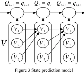
In this simulation experiment, we randomly generated a state node Q and four influence factorsV V V V₁, , ,₂ ₃ ₄. We finally got three factors satisfied the selection condition by Selection algorithm mentioned in section 2. These factors were respectively named

_{V V V}

₁

_{, ,}

₂ ₃ .The other factors

_V

₄ was abandoned, because it does not meet the selection criteria. The final selection results match with the condition for generating random numbers. Therefore it shows that factors selection algorithm has better identification. We obtained three dependencies between adjacent factors by time dependence of the learning algorithm. These dependencies are respectively

1 1 1

t t

V− →V , 1

2 1

t t

V− →V and V3t−1→V1t, and the results show

that the learning algorithm is effective.

When we got the influence factors, dependencies among nods, and various parameters, the final complete model can be constructed. Because the parameters are too more, the CPTs in the model are not listed.

The state prediction model is shown in Figure 3.

Meanwhile, after the study of a random sample of the data, we ultimately got the parameter

_α

which is used in the maintain factor and transfer factor. The average duration for all values of the state node is Ti.

α

is equal

to one, and then we can see that the maintenance factor

and the transfer factor always equal one according to the characteristics of the exponential function. This shows that the state transition probability met invariance in the forecasting model.

B. State Prediction algorithms verification

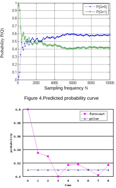
After learning the state prediction model shown in figure 5.1, we give two examples to respectively validate single-step algorithm and multi-step algorithm. In these examples, assume that the current time is t = 0, and value of each node at the current time isQ0=1,V₁0=V₂0=V₃0=0.

Assuming that the distance between the prediction time and the current time is less than or equal to

Δ

t

, thus it would take the single step prediction. Prediction time is credited to t=1. When making single-step prediction, let’s assume that the values of all factors at time t are unknown. According to the results, we draw the prediction probability curve of the state shown in Figure 4. The sampling interval was 100 in the example.It can be seen from the figure that the state prediction probability gradually stabilizes with increase in the sampling frequency. Therefore, the sampling results show that the single-step prediction algorithm has good convergence.

Assuming that the distance between the prediction time and the current time is larger than

Δ

t

, it would take the multi-step prediction. Prediction time is credited to t=T. In the experiment, let T=9 and these time slices be denoted 0,1,2…,8. During the experiment, we recorded each prediction probability of the 9-chip state node. The chart shows that the predict probability gradually decreases and finally fluctuates in the prior probability over time. There is the conclusion that the prediction is

t t

Q =q

1 1

t t

Q₋ =q₋ Q_t₊₁ =q_t₊₁

V

1

V V₁ V₁

2

V V₂ V₂

3

V V₃ V₃

(7)

meaningless when the predicted moment is far away from current. Therefore the algorithm is suitable for short-term forecast.

ACKNOWLEDGMENT

We would like to thank LIU Xuning and HE Dongbin who were collaborators on much of the work reviewed in this chapter. The author was supported by Shijiazhuang University research foundation.

REFERENCES

[1] Murphy Kevin Patrick.Dynamic Bayesian

Networks:Representation, Inference and Learning.University of California,Berkeley, Ph.D thesis. 2002.

[2] Dean T.L,Kanazawa K.Probabilistic temporal

reasioning[A].Mitchell T M,Smith RG.Proc of 7th National

conference on AI[C].Madsion,Wisconsin: AAAI Press.524-528,1988.

[3] Cristina Elena Manfredotti, Modeling and inference with

relational dynamic Bayesian networks, Ph.D thesis October 2009.

[4] Le Song,Mladen Kolar,Eric P.Xing,Time-Varying

Dynamic Bayesian Networks.NIPS,2009.

[5] Xiang Xuan and Kevin Murphy.Modeling changing

dependency structure in multivariate time series.In ICML

24,2007.

[6] Amr Ahmed and Eric P.Xing.Tesla:Recovering

time-varying networks of dependencies in social and

biological studies.Proceeding of the National Academy of

Sciences,in press,2009.

[7] Joshua W.Robinson, Alexander J.Hartemink, Learning

Non-Stationary Dynamic Bayesian Networks.Jorunal of

Machine Learning Research 11:3647-3680,2010.

[8] T.Dean and K.Kanazawa, ”A model for reasoning about

persistence and causation,” Computational

Intelligence,Vol.5,pp.142-150,1989.

[9] Pearl J.Probabilistic Reasoning in Intelligent

System:Networks of Plausible Inference.Morgan

Kaufmann,San Mateo,CA,1988.

[10]Weisheng_Li,Baoshu_Wang.Situation Assessment Based

on Bayesian Networks. SYSTEMS ENGINEERING AND

ELECTRONICS. Vol.25,No.4,2003.

[11]Umnt A.Acar,Guy E.Blelloch,Robert Harper,Jorge

L.Vittes,and Maverick Woo.Dynamizing static algorithms with applications to dynamic trees and history

independence.In ACM-SIAM Symposium on Discrete

Algorithms(SODA),2004.

[12]Darwiche.A. Constant Space Reasoning in Dynamic

Bayesian Networks.Intl. J. of Approximate Reasoning,

26:161–178, 2001.

[13]U. Kjaerulff. dHugin: A computational system for dynamic

time-sliced Bayesian networks.Intl. J. of Forecasting,

11:89–111, 1995.

[14]Pearl J.Bayesian Networks.UCLA Congnitive Systems

Laboratory, Technical Report(R-277), November.2000.

[15]S.Geman and D.Geman. Stochastic relaxation, Gibbs

distributions,and the Bayesian restoration of images,IEEE

Transactions on Pattern Analysis and Machine Intelligence,6:721-741,1984.

[16]Bockhorst J,Craven M,Page D,et al.A Bayesian network

approach to operon prediction. Bioinformatics ,19(10):1227-1235,2003.

Zili Zhang, born in Shijiazhuang, 1981, professor, received the master degree at Yunan University,Kunming, China. The major field of study focus on artificial intelligence .

His current job is teacher. His research interests include data mining and network security.

Hongwei Song was born in 1966, professor, Her research interests include artificial intelligence and network security.

Yan Li, was born in 1981,Master, Her research interests focus on neural compution and wireless sensor networks..

Hao Yang, born in 1990, His research interests focus on data management.

Sampling frequencyN

Pro

ba

bil

ity P(Q)

Figure 4.Predicted probability curve