Abstract—In this paper, B2-spline interpolation technique for Overset Grid Generation and
Finite-Difference Time-Domain (OGG-FDTD) method was developed. B2-spline or biquadratic spline
interpolation offers better accuracy than bilinear interpolation. Two-dimensional (2D) numerical simulations were carried out for electromagnetic (EM) field analysis to measure the scattered fields for an unknown object in free space and dielectric medium. In this work, two antennas were utilised as transmitter and receiver sequentially to transmit microwave pulses and collect the scattered fields for an unknown object in OGG-FDTD lattice. In order to analyse the stability and efficiency of the proposed method, the scattered fields for the unknown object were investigated with error analysis. The results showed that the OGG-FDTD method with B2-spline interpolation gave lower relative error
than bilinear interpolation with 0.0009% of difference in free space, 0.0033% of difference in Case A dielectric medium, 0.236% of difference in Case B dielectric medium, and 0.003% of difference in Case C dielectric medium. Besides, the Mean Square Error (MSE) for the OGG-FDTD method with B2-spline
interpolation was also lower than the bilinear interpolation. Hence, it proves that the OGG-FDTD method with B2-spline interpolation has the ability to measure the scattered fields around an unknown
object accurately. For future work, the proposed method can be applied to inverse scattering to detect and reconstruct buried objects with arbitrary shapes in a complex media.
1. INTRODUCTION
Interpolation has attracted significant interest of researchers due to its potential utility and effectiveness in computer graphics, digital photography, multimedia, geology, agriculture and medical image processing applications [1–4]. Interpolation is the process of defining a function that matches the given data exactly. The function can be utilised to estimate the values that lie between known data points [5, 6]. It also seeks to fill in missing information in some small regions of the whole dataset. This technique can be used to produce a smooth graph of function for measuring or calculating. Besides that, the interpolation method is also useful in image processing for the enhancement of image zooming, reduction, resizing, decomposition, and sub-pixel image registration [7, 8].
There are several interpolation algorithms developed for image processing. Among the famous 2D interpolations are nearest neighbour interpolation [9], bicubic interpolation [10], bilinear interpolation [11], and B-spline interpolation [12–14]. The nearest neighbour interpolation is a simple and fast interpolation method, but the images produced are blurry [13]. On the other hand, bicubic interpolation provides sharper and better images, but it needs a large amount of calculation and takes more computational time [4, 15].
Received 24 May 2018, Accepted 11 August 2018, Scheduled 23 August 2018
* Corresponding author: Shafrida Sahrani ([email protected]).
1 Applied Electromagnetic Research Group, Department of Electrical and Electronic Engineering, Faculty of Engineering, Universiti
In a recently published paper by Azman et al. [16], Overset Grid Generation and Finite-Difference Time-Domain (OGG-FDTD) method with bilinear interpolation technique was used to determine the characteristics of an object (e.g., its shape, location and dielectric properties) in inverse scattering. However, there were some drawbacks of utilising bilinear interpolation technique. The image produced was imprecise and had visualisation, especially for curves images [4, 17, 18]. Therefore, B2-spline
interpolation [19, 20] is proposed to overcome the limitations of bilinear interpolation as it has better accuracy of constructing new data points within the range of a discrete set of known data points.
In this paper, the OGG-FDTD method with B2-spline or biquadratic spline interpolation technique
is developed to measure the scattered field around an unknown object. The performance of this new numerical method is evaluated by using EM field analysis in Transverse Magnetic mode for 2D. The EM field analysis was divided into two parts: Part 1 is the analysis of transmitted and received signals for electric field in free space, and Part 2 is the analysis of transmitted and received signals for electric field in a dielectric medium. Then, the error analysis is used to validate the accuracy of this proposed numerical method with FDTD and OGG-FDTD with bilinear interpolation technique.
2. OVERSET GRID GENERATION AND FINITE-DIFFERENCE TIME-DOMAIN METHOD (OGG-FDTD) IN DIRECT SCATTERING
2.1. Overset Grid Generation (OGG) Method with B2-Spline Interpolation
The overlapping grids method, also known as the Overset Grid Generation (OGG) method, is an automatic overset structured mesh generation and adaption method for computational fluid dynamic (CFD) about three decades ago [21, 22]. This method is used for aerospace, meteorology, biomedical fluid mechanics and aerodynamics applications, such as bodies in the relative motion, parametric studies, and turbomachinery application [23–26].
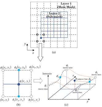
Figure 1(a) shows tha tthe OGG method consists of two meshes. Layer 1 is called the main mesh (dashed line), and it covers the entire computational domain. Layer 2, known as the sub-mesh (solid line), is used to model an unknown object. The position of the sub-mesh is located on top of an overlapped region to form a single grid. The overlapping region between the main mesh and sub-mesh can be obtained by using the B2-spline interpolation technique. This technique used known data values
on the main mesh to estimate the unknown data values on the sub-mesh. The value at the interpolation point is used to transfer inter-grid information and it is recomputed at each time step.
Figure 1(b) is a B2-spline interpolation diagram that is subtracted from Figure 1(a). ∅1, ∅2, ∅3
and ∅4 points are four known value points at the main mesh, while the ∅s point is the unknown value
point at the sub-mesh. Figure 1(c) is a side view of Figure 1(b) atx-y plane with intensity in 2D. The unknown value of ∅s is interpolated by using the∅A and ∅B at y-axis as in Equation (1).
φS =
dj+1−dj
2 (yB−yA)
(ys−yA)2+dB(ys−yA) +φA, j= 0,1,2, . . . , m (1)
where
dj = 0, dj+1 =
2 (φB−φA)
yB−yA −dj, j= 0,1,2, . . . , m
φA =
di+1−di
2 (x2−x1)
(xA−x1)2+di(xA−x1) +φ1
∵di = 0, di+1=
2 (φ2−φ1)
x2−x1 −di, i
= 0,1,2, . . . , n
φB =
di2+1−di2
2 (x4−x3)
(xB−x3)2+di2(xB−x3) +φ3
∵di2 = 0, di2 =
2 (φ4−φ3)
x4−x3 −di2, i2
= 0,1,2, . . . , n
For natural spline, dj = 0, di = 0, and di2 = 0 when j = i = i2 = 0. The unknown value of ∅A is
interpolated by using the known values of ∅1 and ∅2 whereas the unknown value of ∅B is interpolated
(b)
(a)
(c)
Figure 1. Overset grid generation method with B2-spline interpolation model.
2.2. OGG Method Incorporated with FDTD Method and B2-Spline Interpolation in Direct Scattering
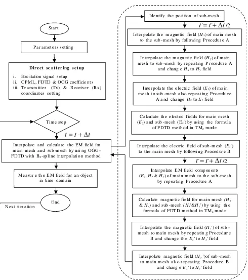
Figure 2 shows a flow diagram of OGG-FDTD with B2-spline interpolation method. All parameters
required in this simulation were declared, and the values were set. Then, the process of measurement for the scattered field was set up.
The EM field components on the main mesh were set asEz,Hx &Hy while those on the sub-mesh were set asEz,Hx &Hy. The magnetic field on the main mesh (Hx) was interpolated to the sub-mesh (Hx) via the B2-spline interpolation technique. This interpolation process is explained in Procedure A:
Procedure A: main mesh to sub-mesh interpolation
(i) In Figure 3(a), the main mesh and sub-mesh points for Hx field were declared as follows: (a) Main-point Hx[m][n2] forφ1(x1, y1) atx-axis
(b) Main-point Hx[m+1][n2] forφ2(x2, y2) at x-axis
(c) Main-point Hx[m][n2+1] forφ3(x3, y3) at y-axis
(d) Main-point Hx[m+1][n2+1] forφ4(x4, y4) at y-axis
(e) Sub-point Hx[i][j]forφs(xs, ys) as the unknown value points at sub-mesh
(ii) The interpolation range forHx component of EM fields was set.
(iii) Referring to Equation (1), the unknown values for φA(xA, yA) were determined by using the known value points, φ1(x1, y1) and φ2(x2, y2) at x-axis on the main mesh through the B2-spline
Ca lculate the electric field s for m a in m esh (Ez) a nd sub -m esh (Ez') by using the for m ula
of F DTD m eth od in TMz m ode Identify the position of sub -m esh
Inter pola te the electric field of sub -m esh (Ez')
to t he m a in m esh by followin g P r ocedur e B
Ca lcu late m a gne ti c field for m a in m esh (Hx
& Hy) a nd sub -m esh (Hx'&Hy') by using th e
for m ula of F DT D m et ho d in TMz m ode Inter polate E M field compon ents (Ez, Hx & Hy) of m a in m esh to the sub -m esh
by r epea ting P r ocedure A
Inter polate the m a gn etic fie ld (Hx') of sub
-m esh t o -m a in -m esh by r epea tin g P r ocedu r e B a nd cha nge th e Ez' t o Hx' fie ld
Tim e step
E nd
Mea sur e th e E M field for a n object in time dom a in
N ext iter a tio n
Inter polate a nd calculat e t he E M fie ld for m a in m esh a nd sub m esh by usi ng OGG -F DTD with B2-sp line inter polati o n m ethod
Sta r t
P a r a m et er s setting
Dire c t s c a t t e ri ng s e tup
i. Exc itation signal setup
ii. CP ML, F DTD & OG G coefficie n t s iii. Tr a nsm itt er (Tx) & Receiver (Rx)
coor dinat es se tting
Inter polate the m a gnetic fie ld (Hx) of m a in m esh
to t he sub - m esh by following P r ocedur e A
Inter pola te the m a gn etic fie ld (Hy) of m a in
m esh t o sub -m esh by r epea ting P r ocedure A a nd chang e Hx to Hy fie ld
Inter pola te the electric field (Ez) of m a in
m esh t o sub -m esh a ls o r epea t ing P r ocedu r e A a nd change Hx t o Ez field
Inter polate m a gn etic field (Hy') of sub -m esh
to m a in m esh a ls o r epea ting P r ocedure B a nd chang e Ez' t o Hy' fie ld
' ' /2
' ' /2
Figure 2. Flow diagram for OGG-FDTD method with B2-spline interpolation in direct scattering.
(iv) Then, the unknown values for φB(xB, yB) were determined by using the known value points, φ3(x3, y3)andφ4(x4, y4) atx-axis on the main mesh through the same interpolation process.
(v) Finally, the unknown values forφs(xs, ys) as the sub-pointHx[i][j]at the sub-mesh were calculated
through the interpolation process by usingφA(xA, yA) and φB(xB, yB) points at they-axis.
(b) (a)
Figure 3. OGG-FDTD method with B2-spline interpolation technique.
process.
The Ez field on the sub-mesh was interpolated into the main mesh, so that the electric field (Ez) on the main mesh is updated. This interpolation process is explained in Procedure B:
Procedure B: sub-mesh to main mesh interpolation
(i) In Figure 3(b), the main mesh and sub-mesh points for Ez field were declared as follows: (a) Sub-point Ez[i][j] forφ1(x1, y1) at x-axis
(b) Sub-point Ez[i+1][j]forφ2(x2, y2) at x-axis
(c) Sub-point Ez[i][j+1] forφ3(x3, y3) at y-axis
(d) Sub-point Ez[i+1][j+1]forφ4(x4, y4) at y-axis
(e) Main-point Ez[m][n]forφs(xs, ys) as the unknown value points at main mesh
(ii) The interpolation range forEz component of EM fields was set.
(iii) Referring to Equation (1), the unknown values for φA(xA, yA) were determined by using the known value points, φ1(x1, y1) and φ2(x2, y2) at x-axis on the sub-mesh through the B2-spline
interpolation.
(iv) Then, the unknown values for φB(xB, yB) were determined by using the known value points, φ3(x3, y3)andφ4(x4, y4) atx-axis on the sub-mesh through the same interpolation process.
(v) Finally, the unknown values for φs(xs, ys) as the main-point Ez[m][n] at the main mesh were
calculated through interpolation process by using the φA(xA, yA) and φB(xB, yB) points at the y-axis.
This algorithm continued until the time-stepping was concluded. Finally, the scattered fields for the unknown object were measured through the Rx antennas.
3. NUMERICAL MODEL AND SIMULATION SETUP
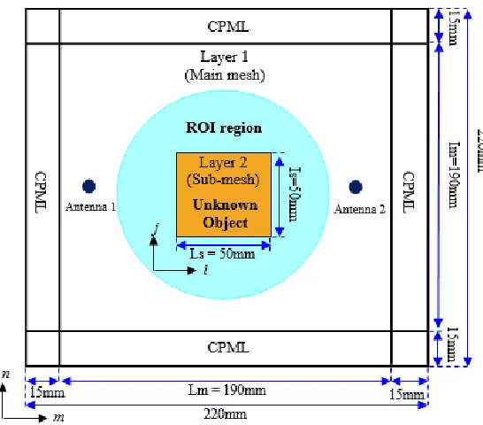
As shown in Figure 4, the 2D numerical image model was implemented to demonstrate the validity of the OGG-FDTD method with B2-spline interpolation in direct scattering. The sub-mesh was set to
Figure 4. Numerical model for OGG-FDTD method with B2-spline interpolation.
There were two antennas utilised in this work; each antenna became the transmitter sequentially to transmit a pulse while the other acted as the receiver to collect the scattered field in the OGG-FDTD lattice. The distance between the two antennas was 170 mm. A sinusoidal modulated Gaussian pulse acted as an excitation signal with centre frequency, fc of 2.0 GHz and bandwidth of 1.3 GHz. This pulse was excited by the transmitter into the OGG-FDTD lattice. The FDTD lattice environment was surrounded by the Convolution Perfectly Matched Layer (CPML) with a thickness of 15 mm to prevent the reflection of the signal at the boundary of the environment.
4. RESULTS AND DISCUSSION
In this section, a preliminary study on the performance of OGG-FDTD method with B2-spline
interpolation in direct scattering was evaluated. The analysis of electromagnetic field for an unknown object was separated into two parts; free space and dielectric medium. All simulation works were carried out by using processor IntelRCore TMi7-6500U 2.5 GHz, 64 bit operating system and 12 GB RAM.
4.1. Analysing the Electromagnetic Field for an Unknown Object in Free Space
The dielectric properties for the background, Region of Interest (ROI) and object in a free space were set up based on Table 1.
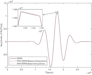
Figure 5 and Figure 6 illustrate the comparison for transmitted and received signals for electric field in free space by using the FDTD method, OGG-FDTD method with bilinear interpolation, and
Table 1. Electrical profiles for modelling setup in free space.
Layer Media Region Size εr (F/m) σ (S/m)
Layer 1 (Main mesh) Background 190 mm×190 mm 1.00 0.00
ROI 50 mm (radius) 1.00 0.00
Figure 5. Transmitted signal for electric field in free space.
Figure 6. Received signal for electric field in free space.
OGG-FDTD method with B2-spline interpolation. The solid line represents the FDTD method; dashed
line represents the FDTD method with bilinear interpolation; dotted line represents the OGG-FDTD method with B2-spline interpolation. These three methods reached the maximum amplitude
In order to analyse the efficiency of the proposed method, the error analysis for received signal was calculated as follows:
RelativeError = |Ez(t)−E0(t)| E0(t)
(2)
MSE = 1 N
N
i=1
[Ez(t)−E0(t)]2 (3)
where E0(t) is the electric field in FDTD lattice, Ez(t) the electric field in OGG-FDTD lattice with
bilinear interpolation or OGG-FDTD lattice with B2-spline interpolation, and N the total number of
time steps.
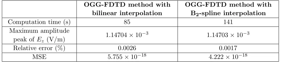
Table 2. Computation time and error analysis for received signal in free space.
OGG-FDTD method with bilinear interpolation
OGG-FDTD method with B2-spline interpolation
Computation time (s) 85 141
Maximum amplitude
peak ofEz (V/m) 1.14704×10
−3 1.14703×10⁻³
Relative error (%) 0.0026 0.0017
MSE 5.755×10⁻¹⁸ 4.222×10⁻¹⁸
Table 2 presents the computation time and error analysis for received signals in free space. The maximum amplitude peak of electric field,Eo(t), for FDTD method was 1.14701×10⁻³V/m, and it was used as a reference in this analysis. The OGG-FDTD method with B2-spline interpolation showed lower
relative error than OGG-FDTD method with bilinear interpolation of 0.0009% difference. Additionally, the MSE for OGG-FDTD method with B2-spline interpolation was also lower than OGG-FDTD method
with bilinear interpolation. The results indicate that OGG-FDTD method with B2-spline interpolation
can measure the scattered fields in free space efficiently as compared to bilinear interpolation. However, the OGG-FDTD method with B2-spline interpolation required more computational time than the
OGG-FDTD method with bilinear interpolation. This is due to the procedure for deriving the coefficients of B2-spline interpolation which use information from all data points, while bilinear interpolation only
uses information from neighbouring data points with straight lines.
4.2. Analysing Electromagnetic Field for an Unknown Object in a Dielectric Medium
In order to analyse the stability and accuracy of the proposed method, different types of dielectric medium for an unknown object were described in Case A, Case B, and Case C. The unknown object was embedded in a circular region of interest (ROI) with free space as the background medium.
4.2.1. Case A: Dielectric Medium for Square Object Similar to ROI
The sub-mesh is modelled as a square object. The dielectric properties for square object were set similar to ROI. The main mesh was set to 190 mm×190 mm grids and the sub-mesh set to 50 mm×50 mm grids. The electrical profiles for Case A are summarised in Table 3.
Figure 7 illustrates the comparison for transmitted and received signals in Case A dielectric medium by using the FDTD method, OGG-FDTD method with bilinear interpolation, and OGG-FDTD method with B2-spline interpolation. The FDTD method is represented by solid line, OGG-FDTD method
with bilinear interpolation by dashed line, and OGG-FDTD method with B2-spline interpolation by
dotted line. The three methods reached the maximum amplitude peak ofEz-field at 1.19244 ns for the transmitted signal and 2.42183 ns for the received signal.
OGG-FDTD method with bilinear interpolation
OGG-FDTD method with B2-spline interpolation
Computation time (s) 86 144
Maximum amplitude
peak ofEz (V/m) 5.9573×10−
4 5.9575×10⁻⁴
Relative error (%) 0.005 0.00167
MSE 3.181×10⁻¹⁸ 1.002×10⁻¹⁸
Figure 7. Transmitted and received signals for electric field in Case A.
free space. The relative error for the received signal in Case A dielectric medium was compared among FDTD method, OGG-FDTD method with bilinear interpolation, and OGG-FDTD method with B2
-spline interpolation. The electric field,E0(t), calculated by the FDTD method was 5.9576×10⁻⁴V/m,
and it was used as reference in this analysis. The results show that the OGG-FDTD method with B2
-spline interpolation can measure the scattered field around the unknown object efficiently by producing lower relative error than the OGG-FDTD method with bilinear interpolation. The difference of relative error between these two methods was 0.0033% in Case A. Besides, the MSE of OGG-FDTD method with B2-spline interpolation was lower than bilinear interpolation with a difference of 2.179×10⁻¹⁸ in
4.2.2. Case B: Dielectric Medium for Square Object Different from ROI
The sub-mesh is modelled as a square object similar to Case A. In this case, the dielectric properties for the square object were set differently from ROI. The electrical profiles for Case B numerical model are summarised in Table 5.
Table 5. Electrical profiles for Case B.
Layer Media Region Size εr (F/m) σ (S/m)
Layer 1 (Main mesh) Background 190 mm×190 mm 1.00 0.00
ROI 50 mm (radius) 9.98 0.18
Layer 2 (Sub-mesh) Square Object 50 mm×50 mm 21.45 0.46
Figure 8 illustrates the transmitted and received signals for electric field in Case B. Figure 8(a) shows that these three methods reached the maximum amplitude peak at 1.19244 ns for the transmitted signal. However, for the received signal, they reached the maximum amplitude peak of E-field at a different time as shown in Figure 8(b). The OGG-FDTD method with bilinear interpolation and OGG-FDTD method with B2-spline interpolation reached the maximum amplitude peak of Ez-field at
2.65522 ns with the FDTD method at 2.66677 ns.
(b) (a)
Figure 8. (a) Transmitted signal, (b) received signal for electric field in Case B.
Table 6 shows the computation time and error analysis for the received signal in Case B. Case B requires more computation time than Case A with 35 seconds of difference for the OGG-FDTD method with bilinear interpolation and 37 seconds for the OGG-FDTD method with B2-spline interpolation.
The amplitude ofEz-field for the received signal in Case B is lower than Case A because the dielectric properties for the unknown object in Case B are higher than Case A. To investigate the accuracy of the proposed method, the relative error and MSE analysis were calculated based on Equations (2) to (3). The FDTD method was used as reference in this analysis with electric field,E0(t) = 2.9821×10⁻⁴V/m.
The results showed that the relative error for OGG-FDTD method with B2-spline interpolation was
lower than bilinear interpolation with 0.1246% of difference. Besides, the MSE for the OGG-FDTD method with bilinear interpolation was 4×10⁻¹³ higher than the OGG-FDTD method with B2-spline
4.2.3. Case C: Dielectric Medium for Circular Object Different from ROI
The sub-mesh is modelled as a circular object. In this case, the dielectric properties for the circular object were set differently from ROI. The main mesh was set to 190 mm×190 mm grids and the sub-mesh set to 24 mm×24 mm grids. The electric profiles for Case C are summarised in Table 7.
Table 7. Electrical profiles for Case C.
Layer Media Region Size εr (F/m) σ (S/m)
Layer 1 (Main mesh) Background 190 mm×190 mm 1.00 0.00
ROI 50 mm (radius) 9.98 0.18
Layer 2 (Sub-mesh) Circular Object 10 mm (radius) 35.25 1.12
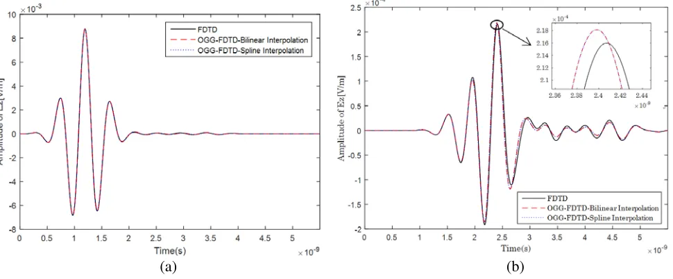
Figure 9 illustrates the transmitted and received signals for electric field in Case C. Figure 9(a) shows that these three methods reached the maximum amplitude peak at 1.19244 ns for the transmitted signal, but the values of Ez-field are different. The maximum amplitude peaks of transmitted signal for OGG-FDTD method with bilinear and B2-spline interpolations are similar at 8.76899×10⁻³V/m
while for the FDTD method, the value is 8.76894×10⁻³V/m. Figure 9(b) illustrates the received signal for electric field by utilising the three methods. The OGG-FDTD method with bilinear and B2-spline
interpolations reached the maximum amplitude peak ofEz-field at 2.39872 ns, while the FDTD method at 2.40796 ns.
(b) (a)
Table 8. Computation time and error analysis for received signal in Case C.
OGG-FDTD method with bilinear interpolation
OGG-FDTD method with B2-spline interpolation
Computation time (s) 29 45
Maximum amplitude
peak ofEz (V/m) 2.18163×10
−4 2.18158×10⁻⁴
Relative error (%) 1.007 1.004
MSE 5.1545×10⁻¹¹ 5.1502×10⁻¹¹
Table 8 shows the computation time and error analysis for the received signal in Case C. The computation time for Case C is lower than Case A and Case B because the object size and interpolation for the sub-mesh are smaller than that of Case A and Case B. The amplitude ofEz-field for the received signal in Case C is also lower than Case A and Case B because the dielectric properties for the unknown object in Case C are higher than that of Case A and Case B.
In this study, the relative error and MSE analysis were calculated to investigate the stability and accuracy of the proposed method. The FDTD method was used as reference in this analysis. It was found that the percentage of relative error and MSE for the OGG-FDTD method with B2-spline
interpolation were lower than that of bilinear interpolation. Hence, it can be said that the OGG-FDTD method with B2-spline interpolation can measure the scattered field around an unknown object more
accurately than the bilinear interpolation.
5. CONCLUSION
The OGG-FDTD method with B2-spline interpolation method was applied to measure the scattered
fields around an unknown object. The signal analysis for electromagnetic field proved that the proposed numerical method was able to obtain the transmitted and received signals in free space and dielectric medium. For further investigation, different types of dielectric medium for an unknown object were analysed in Case A, Case B, and Case C. The relative error and MSE for the proposed method were lower than the OGG-FDTD method with bilinear interpolation. Thus, it can be concluded that the proposed numerical method can measure the scattered fields around an unknown object accurately. For future research works, the proposed method can be applied to inverse scattering to determine the characteristic of buried objects (e.g., its shape, size, location, and dielectric properties).
ACKNOWLEDGMENT
This research was supported by Dana Pelajar PhD (DPP) Grant F02/DPP/1602/2017, Universiti Malaysia Sarawak (UNIMAS), Ministry of Education Malaysia.
REFERENCES
1. Mahajan, S. H. and V. K. Harpale, “Adaptive and non-adaptive image interpolation techniques,”
International Conference on Computing Communication Control and Automation (ICCUBEA), IEEE, 772–775, 2015.
2. Sinha, A., M. Kumar, A. K. Jaiswal, and R. Saxena, “Performance analysis of high resolution images using interpolation techniques in multimedia communication system,”Signal & Image Processing, Vol. 5, No. 2, 39, 2014.
integer scaling ratio,” Quantum Information Processing, Vol. 14, No. 11, 4001–4026, 2015.
10. Warbhe, S. and J. Gomes, “Interpolation technique using non-linear partial differential equation with edge directed bicubic,”International Journal of Image Processing (IJIP), Vol. 10, No. 4, 205, 2016.
11. Iwamatsu, H., R. Fukumoto, M. Ishihara, and M. Kuroda, “Comparative study of over set grid generation method and body fitted grid generation method with moving boundaries,”in Antennas and Propagation Society International Symposium, AP-S 2008. IEEE, 1–4, 2008.
12. Spath, H., Two Dimensional Spline Interpolation Algorithms, 1–68, United States of America: A K Peters, Wellesley, Massachusetts, 1995.
13. Han, D. Y., “Comparison of commonly used image interpolation methods,” in Proceedings of the 2nd International Conference on Computer Science and Electronics Engineerings (ICCSEE), 1556– 1559, 2013.
14. Xia, P., T. Tahara, T. Kakue, Y. Awatsuji, K. Nishio, S. Ura, T. Kubota, and O. Matoba, “Performance comparison of bilinear interpolation, bicubic interpolation, and B-spline interpolation in parallel phase-shifting digital holography,”Optical Review, Vol. 20, No. 2, 193–197, 2013. 15. Sinha, A., “Study of interpolation techniques in multimedia communication system-a review,” 2015. 16. Azman, A., S. Sahrani, K. H. Ping, and D. A. A. Mat, “A new approach for solving inverse scattering problems with overset grid generation method,” TELKOMNIKA (Telecommunication Computing Electronics and Control), Vol. 15, No. 1, 820–828, 2017.
17. Kaur, K., I. Kaur, and J. Kaur, “Survey on image interpolation,”International Journal of Advanced Research in Computer Science and Software Engineering, Vol. 6, No. 5, 613–616, 2016.
18. Patel, V. and K. Mistree, “A review on different image interpolation techniques for image enhancement,” International Journal of Emerging Technology and Advanced Engineering (IJETAE), Vol. 3, 129–133, 2013.
19. Boor, C. D.,A Practical Guide to Spline, Springer-Verlag, 1978.
20. Schumaker, L. L., Spline Functions: Computational Methods, Society for industrial and applied mathematics (SIAM), 2015.
21. Thompson, J. F., Z. U. Warsi, and C. W. Mastin, Numerical Grid Generation: Foundations and Applications, Vol. 45, North-holland Amsterdam, 1985.
22. Thompson, J. F., B. K. Soni, and N. P. Weatherill, Handbook of Grid Generation, CRC Press, 1998.
23. Castillon, L. and G. Legras, “Overset Grid Method for simulation of compressors with nonaxisymmetric casing treatment,” Journal of Propulsion and Power, Vol. 29, No. 2, 460–465, 2013.
24. Renaud, T., A. L. Pape, and S. P´eron, “Numerical analysis of hub and fuselage drag breakdown of a helicopter configuration,” CEAS Aeronautical Journal, Vol. 4, No. 4, 409–419, 2013.
26. Wiart, L., O. Atinault, D. Hue, R. Grenon, and B. Paluch, “Development of NOVA aircraft configurations for large engine integration studies,”33rd AIAA Applied Aerodynamics Conference, 2015.