A Cooperative and Heuristic Community
Detecting Algorithm
Ruixin Ma
School of software, Dalian University of Technology, Dalian, China Email: [email protected]
Guishi Deng and Xiao Wang
School of Management Science and Engineering, Dalian University of Technology, Dalian, China Email: [email protected], [email protected]
Abstract—This paper introduces the concept of community seed, vector and relation matrix. In terms of the relation similarity between free vertices and the existing communities, we put vertices into different groups. A minimum similarity threshold is proposed to filter which gives a method to find the vertices located at the overlapped area between different communities. This paper analyzes a series of network dataset and proves that our algorithm is able to accurately find communities with high cohesion and weak coupling. We use a variety of test to demonstrate that our algorithm is highly effective at detecting community structures in both computer-generated and real-world networks.
Index Terms—community seed; relation matrix; minimum similarity threshold; overlapped area; high cohesion and weak coupling
I. INTRODUCTION
Network has attracted considerable recent attention as one of the most powerful mathematical presentation for complex systems. Network ideas have been applied with success to topics as diverse as scientific citation and collaboration [1], epidemiology [2], ecosystems, to name but a few. Previous study indicates that large complex networks have statistical features such as small-world phenomenon [3], isomerism [4], clustering, scale-free [5]. According to the recent research, complex networks also have obvious community structures [6]. Community structure is the reflection of networks’ modularization and heterogeneity; it tells us that the real world is combined by all sorts of vertices. It is of vital significance to deeper study the community structures which hidden behind the complex networks, as well as to intellectually mine them. For example, communities in social networks can be used to find vertices of similar interests and social context; classifying the pages on world wide web is good to improve the search efficiency and accuracy, and help to implement the function of information filtering, hot spots tracking, news analyzing and so on; the discovery of community in biochemistry networks and electronic networks is useful to find the function-related structure units. Finding these communities are not only helps to
reveal how the high cohesion and loose coupling community structures are combined, but also helps people to better understand the distinctive characteristics of structures and functions in different levels of the system.
Community detecting can be defined as: finding the vertices with similar characteristics in the complex network and artificially put them into a virtual group. Vertices in the same group have tightly connections while vertices in different groups have sparse connections [7][8]. After division we get a high cohesion and loose coupling system. The feature of community in complex network is similar to the clustering in data mining, so this feature is also called clustering. The ability to find and analyze communities in complex network can provide invaluable help in understanding and visualizing the structure of complex networks [9-20]. In this paper, we show how this can be achieved.
Classical community discovery algorithms (CDA) include, G-N algorithm [10][15], label propagation algorithm [11-13], the CDA based on dynamical similarity[14], to name but a few. With the development of swarm intelligence, some scholars also came up with the idea of CDA based on genetic algorithm (GA) [16-19] and CDA based on particle swarm optimization (PSO)[20-22]. According to the operational solution strategies, the existing CDAs can be divided into two classes, heuristic CDA and optimal CDA. This paper is enlightened both by the thoughts in PSO and by the cooperative thoughts in CF, we entitled it as cooperative and heuristic CDA (CHCDA). Experimental results in section 4 show that the applications can effectively lower the algorithm’s time complexity with good practicality and applicability.
II.PRELIMINARIES
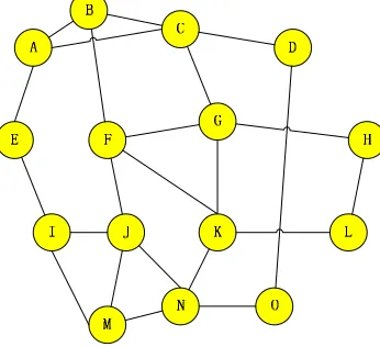
Figure 2. A simple undigraph. Figure 1. A small artificial network.
for the community seed; then we compare the similarities between free vertices and the existing community. In this paper, we use vertices’ degree as the weight of core level, take the core vertex as the best particle, look for and detect the community structures in complex networks. A. Relation matrix
Assume that the network we studied has n nodes, A is the adjacent matrix and R is the relation matrix.
Rn=An+En (1) From the above formula we can see, the difference between A and R is, the diagonal elements in adjacent matrix is Ai,i=0 while the relation matrix is Rj,j=1.
We use Figure 1to illustrate how CHCDA works. The theory of “Six Degrees of Separation” tells us that people who have same friends are much easier to become friends themselves than people who are randomly picked up from the society. Before theorem one, we define the concept of common neighbor and the concept of people with similar social relationships.
Definition 1: Common neighbor. If node a has edges to both node i and j, a is i and j’s common neighbor.
Definition 2: Similar social relationship. If i and j have many common neighbors and exceed a minimum threshold, we call i and j have similar social relationships.
In this paper, we use relation similarity to weigh how close the nodes’ are. According to the description above we get Theorem 1.
Theorem 1: In network N, We know that A and B are friends, B and C are friends, D and E are randomly chosen from N. We say that A and C are much easier to become friends than D and E. In other words, similarity(A,C)>>similarity(D,E)。
Graph theory is always used to solve the problems in network; the problem described above is equal to calculate the probability of triangle formation in an undigraph. In other words, we need to prove that the probability of Triangle (A,B,C)>>Triangle(D,B,E).
Proof:
(1) Construct a simple undigraph as Figure 2 shows; (2) Set node B as a triangle vertex;
(3) If nodes A and C are both B’s nearest neighbor, the probability of A, B and C to form a triangle is 50%; (4) If we randomly choose another two nodes D and E
from the graph, the probability of B, D and E to form a triangle is 0.5*0.5*0.5=0.125;
(5) Therefore, the similarity between A and C is much higher than D and E.
Inference 1: Nodes who have similar social relationship are more probable belong to the same community.
We construct the relation matrix in accordance with Figure 1 as below.
⎥ ⎥ ⎥ ⎥ ⎥ ⎥ ⎥ ⎥ ⎥ ⎥ ⎥ ⎥ ⎥ ⎥ ⎥ ⎥ ⎥ ⎦ ⎤ ⎢ ⎢ ⎢ ⎢ ⎢ ⎢ ⎢ ⎢ ⎢ ⎢ ⎢ ⎢ ⎢ ⎢ ⎢ ⎢ ⎢ ⎣ ⎡ = 1 1 1 0 0 0 1 0 0 0 0 0 1 1 1 0 0 0 0 0 0 0 0 0 1 1 1 0 0 0 0 0 0 0 0 0 0 0 0 1 0 1 1 1 1 0 0 0 0 0 0 0 1 1 1 0 0 0 0 0 0 0 0 1 1 1 1 0 0 0 0 0 1 0 0 1 1 1 1 1 0 0 0 0 0 1 0 1 0 0 1 1 1 1 1 1 0 0 0 1 0 0 0 1 1 1 1 1 0 0 0 0 0 0 0 1 1 1 0 0 0 0 0 0 0 0 0 1 1 0 1 1 0 0 0 0 0 0 0 1 1 0 1 1 Matrix
By analyzing the matrix we know, the ith row of matrix represents the relation vector of i. As a result, we get the degree of i as formula 2 shows.
1 1 , − =
∑
= n j j i i MatrixDegree (2)
By calculating the cosine similarity between relation vectors, we can find the most similar neighbor for each target vertex or community.
B. Community vector
eigenvector of community is combined by the relation vectors of the inner vertices. In this paper, we come up with two methods to demonstrate community eigenvectors.
• Binary vector representation
This method use binary numbers 0 and 1 to represent the community eigenvectors.
For example, the relation matrix of Figure 1 is Matrix, the relation vector of vertex i is Matrixi. We use VSNto represent the eigenvector of community SN, and the vector length is 12, the initial value of VSN is 0. The binary vector representation method can be described as below.
foreach node i in SN
i SN
SN V Matrix
V = ∪ (3) VSN(i)=1 means that there is more than one edge to vertex i, while VSN(i)=0 means none. This method is only able to show whether there is an edge to i or not, but not able to count how many. Therefore, we put forward another method to represent the community’s relation eigenvector.
• Relation weighted vector representation
This method is able to count the number of edges direct to the target vertex i, which to some extent reflects i’s attraction. We use SNi(a) to represent the number of edges in community SNi to vertex a. The larger of SNi(a), the bigger of a’s attraction. The calculation of relation weighted vector can be described as below.
foreach node i in SN
VSN=VSN+Matrixi (4) In this paper, the addition rules are as same as in math. Use Figure 1 as example, vertex 4 and 5belong to SN1. If we use binary representation, VSN1=V4∪V5= <1,1,1,1,1,
1,0,0,1,0,1,0>. This result tells us that there are edges direct to vertices 1, 2, 3, 4, 5, 6, 9, 11 in the network, but we do not know how many. If we use relation weighted representation method, VSN1= V4+V5=<2,2,2,2,2,1,0,0,
1,0,1,0>, it tells us that for this moment, there are two edges direct to vertices 1, 2, 3, 4, 5, and one edge direct to vertices 6, 9, 11.
Community vector vividly shows the relationship between vertices in the community, which makes it possible to weigh the similarity between free vertices and the existing communities. Besides, it provides an interface for the application of CF to CDA.
C. Community seed
Based on thoughts in multi-function optimization, the best particle leads the rest ones to locate at the most suitable place[23]. Low degree means the vertex locate at the margin place while high degree means it locates at the core position. Community seed is the best local one in one community. We define the concept of community seed and free members as blew.
Definition 3: Community seed. If vertex a is the first member of a community, it leads the following members
to locate around it. The number one vertex becomes the seed of this community.
Definition 4: Free members. The remained nodes in Ldegree that haven’t been divided into communities are called free members.
The steps to choose community seed are as below. Step 1: All vertices are sorted in decreasing order of degrees which constitute a list Ldegree.
Step 2: The set of community seeds S is initially set to empty.
Step 3: Vertices in Ldegree are checked in turn from the beginning to the end of the list. If vertex i does not have connection with the existing communities{SN}, it becomes a new seed and is added to S; if not, calculate the similarity between i and SN and if similarity(i, SN)< δ, i become a new seed and be added to S; else if similarity(i, SN)>δ, i becomes a member of SN.
Because vertices with higher degrees are checked first, the community seed in each community must be the one with best location. These community seeds respectively guide the rest nodes in the same network to locate at the multiple optima.
The similarity between community SN and vertex i is calculated as formula (5) shows.
Sim(S,i)=cos(S,i)=
i S
i S
V V
V V
⋅ ⋅
(5)
When the scale of network changes, it become necessary to change the minimum similarity threshold δ. The larger of the network scale, the more complex of the relationship between vertices. The largest number of edges in a network who have n vertices is (n^2-n)/2, which means one vertex has a maximum (n-1) neighbors. This paper uses relation matrix to represent the relationship between vertices in a network, every vertex has relation to itself which makes the biggest relation number to n. The principle of cosine similarity is that the more of the common neighbors that a pair of vertices have, the closer of the relationship between them. In a social network with n vertices, the maximum of the common neighbors is n, in other words, if two vertices have n common neighbors, the similarity between them must be 1, so we set the unit of minimum similarity threshold as 1/n.
III.CHCDA
In this algorithm, the number of seeds determines the number of communities in the entire network. As a result, we don’t need to artificially set the number of communities.
A. Description of community division
We still use Figure 1 to illustrate how this algorithm works out. For Figure 1, Ldegree=<5,6,4,11,1,2,7,
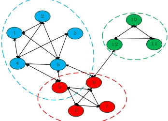
Figure 3. Division of binary community vector representation
Figure 5. Divided social structure of the network in figure 1.
Figure 6. Division results of nodes in Zachary Club Figure 4. Division of relation weighted community vector
representation.
Figure 3 is the dividing result of binary representation and Figure 4 is the dividing result of relation weighted representation.
The green dotted line in Figure 3 and Figure 4 is the line of minimum similarity threshold. Compare the results of different community representations, we can see that they get the same community structure, but the relation weighted representation can effectively expand the elasticity of relations between nodes and reduce the fuzzification of node’s position.
Besides, there is a distinctive node in figure 4, node 9 belongs to both A and B. However, the similarity between community B and 9 is much higher. We call node 9 the contactor of A and B. Figure 5 shows the dividing results of relation weighted representation.
B. Procedure of cooperative CDA
Step 1: Construct the adjacent map for network N; Step 2: Build the relation matrix;
Step 3: Sequence the vertices in network N and build up Ldegree;
Step 4: Look for the community seeds, define the community vectors.
Step 5: Divide vertices into different communities.
IV.EXPERIMENTAL RESULTS
, We apply CHCDA to the dividing of Zachary club and dolphins network to test the feasibility of our algorithm.
A. Zachary Club Network
Zachary Club is a one of the most classical network for analyzing network structures. In 1970s, Wayne Zachary took three years to observe the social relationships of members in a US college’s karate club, after then he constructed the Zachary’s karate club network. The dataset includes 34 nodes and 78 edges, each node represents one member in the club, and edges state the relationship between members. In the procedure of investigation, he found that the director and the coach had disputes with each other about charging problems which result in the whole club break into two parts. The manager and the coach separately became the head of one part. In Figure 6, different colors represent members in different groups. As a real social network, Zachary club is often used to test the efficiency of community discovery algorithm.
Using CHCDA, we firstly construct the relation map of Zachary club. The degree ranking list is Ldegree=< 34, 1,
33, 3, 2, 4, 32, 9, 24, 6, 7, 8, 14, 15, 28, 30, 31, 5, 11, 20, 25, 26, 29, 10, 13,16,17,18,19,21, 22, 23, 27, 12>,δ =1/34. During the test, we use relation weighted representation to illustrate how this algorithm works well.
Figure 7. CHCDA division results for Zachary Club
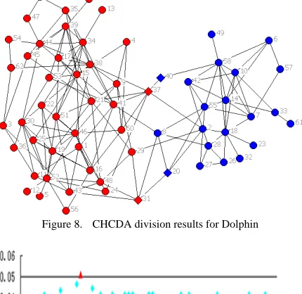
Figure 8. CHCDA division results for Dolphin
Figure 9. Division results of nodes in Dolphin
B. Dolphins Network
Dolphin network is also a common dataset in the study of social networks. Lusseau and his fellows conduct systematic surveys about dolphins in Doubtful Sound, Fiordland, New Zealand. The survey course constantly remains over 7 years and covers the entire home range of Doubtful Sound population which includes 62 vertices and 159 edges. In Figure 8, each vertex represents a dolphin; a link means two dolphins have regular contact. We set the minimum similarity as 1/62 and get Figure 9.
Figure 8 shows that the entire network is divided into two parts. Besides, there are some special dolphins locate at the overlapped area, such as vertex 20, 31 and 37.
Individuals who lie on the boundaries of communities become bridge between unconnected communities. They play important roles in the procedure of information spreading. The discovery of connectors has great value to promote the communication and interaction between communities, especially in the E-commence and citation network.
V.CONCLUSION
In this paper, we have analyzed the problem of detecting community structure in networks. During the research, we come up with a cooperative community detecting algorithm based on the ideas in multi-model optimization. We have three innovation points in this paper: (1) Introduce the concept of community seed, declare that community seeds guide the rest individuals to locate at the multiple optima. (2) Put over the idea of relation matrix, use relation similarity to weigh the social intimacy between nodes. (3) Apply CF’s thoughts to community discovery; find the contactors between different communities. Those three characteristics enable the CHCDA algorithm efficiently finds the potential communities in large complex network.
Follow-up works include formulate the minimum similarity threshold and choose suited community vector representation for different social networks.
REFERENCES
[1] M. E. J. Newman. “Finding community Structure in Networks Using the Eigenvectors of Matrices.” Physics Review E. 2006, 1–22.
[2] S. Boccaletti, V. Latora, Y. Moreno, M. Chavez, and D.-U. Hwang, “Complex Networks: Structure and Dynamics.” Physics Reports 424, 2006, 175–308.
[3] Watts D J, Strogatz S H. “Collective Dynamics of Small- World’ Networks.” Nature, 1998, 393(6638): 440-442. [4] Duan Xiao-dong, Wang Cun-rui, Liu Xiang-dong. “Web
Community Detection Model Using Particle Swarm Optimization.” Computer Science, 2008, 35(3): 18-22. [5] Albert R, Jeong H, Barabasi AL. “The Internet’s Achilles
Heel: Error and Attack Tolerance of Complex Networks.” Nature, 2000, 406(2115): 378-382.
[6] Barabasi AL, Albert R. “Emergence of Scaling in Random Networks.” Science, 1999, 286(5439):509-512.
[7] Guimera` R, Amaral L. A. N. “Functional Cartography of Complex Metabolic Networks.” Nature, 2005, 433(7028): 895-900.
[8] Palla G, Der′enyi I, Farkas I,Vicsek T. “Uncovering the Overlapping Community Structure of Complex Networks in Nature and Society.” Nature, 2005, 435(7043): 814-818. [9] HE Dong-Xiao, ZHOU Xu, WANG Zuo, ZHOU Chun-Guang, WANG Zhe, JIN Di. “Community Mining in Complex Networks—Cluster Genetic Algorithm.” ACTA AUTOMATICA SINICA, 2010, 36(8): 1160-1170. [10]Girvan M,Newman M E J. “Community Structure in Social
and Biological Networks”. Proceedings of the National Academy of Sciences of the United States of America, 2002, 99(12): 7821-7826
[12]Barber M J,Clark J W. “Detecting Network Communities by Propagating Labels Under Constraints.” Physical Review E, 2009, 80(2): 026129.
[13]Leung I X Y,Hui P,Lio` P,Crowcroft J. “Towards Real-time Community Detection in Large Networks.” Physical Review E,2009,79(6):066107.
[14]Zhang Y Z, Wang J Y, Wang Y,Zhou L Z. “Parallel Community Detection on Large Networks with Propinquity Dynamics.” In: Proceedings of the 15th ACM SIGKDD International Conference on Knowledge Discovery and Data Mining. Paris, France: ACM, 2009, 997-1006.
[15]Newman M E J. “Fast Algorithm for Detecting Community Structure in Networks.” Physical Review E,2004, 69(6): 066133.
[16]Liu X, Li D Y, Wang S L, Tao Z W. “Effective Algorithm for Detecting Community Structure in Complex Networks Based on GA and Clustering.“ In: Proceedings of the 7rded International Conference on Computational Science. Beijing, China, Springer, 2007. 657-664.
[17]Gog A, Dumitrescu D, Hirsbrunner B. “Community Detection in Complex Networks Using Collaborative Evolutionary Algorithms.” In: Proceedings of the 9thed European Conference on Artificial Life. Lisbon, Portugal: Springer, 2007. 886-894.
[18]Tasgin M, Herdagdelen A, Bingol H. “Community Detection in Complex Networks Using Genetic Algorithms.” http://arxiv.org/abs/0711.0491, 2010.
[19]Pizzuti C. “A Genetic Algorithm for Community Detection in Social Networks.” In: Proceedings of the 10thed Inter-national Conference on Parallel Problem Solving from Nature. Dortmund, Germany, Springer, 2008. 1081-1090. [20]DAI Fei-fei, TANG Pu-ying. “Community Structure
Detection in Complex Networks Using Particle Swarm Optimization Algorithm.” Computer Engineering and Applications, 2008, 44(22): 56-58.
[21]GAO Chun-tao. “Research on Particle Swarm Optimization and Its Application.” Journal of Harbin University of Commerce (Natural Sciences Edition). 2010, 26(4): 442-445.
[22]X. Li. “Adaptively Choosing Neighborhood Bests using Species in A Particle Swarm Optimizer for Multimodal Function Optimization,” Proceedings of Genetic and Evolutionary Computation Conference, 2004, 105-116. [23]Li, J.P., Balazs, M.E., Parks, G. and Clarkson, P.J. “A
Species Conserving Genetic Algorithm for Multimodal Function Optimization.” Evolutionary Computation. 2002, 10(3): 207–234.
Ruixin Ma, (1975--). Lecturer of Dalian University of Technology. Research area: E-commence, community discovery and swarm intelligence.
Guishi Deng, (1945--). Professor of Dalian University of Technology. Research area: E-commence, decision analysis and analysis of complex system.