An Efficient Finite-Input Receding Horizon Control Method and Its Application for the Pneumatic Hopping Robot

An Efficient Finite-Input Receding Horizon

Control Method and Its Application for the

Pneumatic Hopping Robot

Jian Wu

Engineering Department, Omron Oilfield and Marine, Houston, TX 77088, USA Email: [email protected]

Sherif Abdelwahed

Electrical and Computer Engineering Department, Mississippi State University, USA Email: [email protected]

Abstract— In this paper, a finite-input receding horizon

controller (FIRHC) is proposed as motivated by the need to use solenoid valves to control the motion of a pneumatic hoping robot. The controller aims to the application on switching control systems in which only a finite number of control inputs are available. The controller utilizes a model to predict system behavior along a finite forward horizon, and establishes an optimization problem, and then finds an optimal control sequence that gives the optimal cost and ultimately only the first element of the sequence is applied at each time step. The stability issue of the controller is discussed as a terminal equality constraint is added. Since only finite discrete inputs exist, the analytical solution is usually not possible to achieve, and exhaustive search was generally the approach to get the optimal control input. As is known, the exhaustive search becomes computationally prohibitive with an increasingly long horizon. An efficient modified depth first search algorithm is proposed, namely, sorted depth first search (sDFS). It preserves the completeness of exhaustive search, while significantly reducing time and space complexity. The whole approach is applied to a pneumatic hopping robot system where the motion control is re-formulated as an explicit energy regulation problem. The control goal is to maintain the system energy at a desired level. An additional example on a three tank control system is used to further illustrate the efficiency of sDFS method on the system with possession of a relatively large amount of modes. Simulation results demonstrate the effectiveness of the proposed method.

Index Terms—receding horizon control, switching systems, finite control set, sorted depth first search, energy regulation, hopping robot

I. INTRODUCTION

In this paper, we introduce a feasible and efficient control strategy to regulate the oscillatory motion of a pneumatic hopping robot. Because pneumatic actuators can provide much higher power-to-weight ratio than their electrically actuated competitors, they have been used directly as legs to drive a legged-robot since late 1980s [1]. In the work of Binnard [2], a small six-legged

pneumatic walking robot was designed using customized lightweight pneumatic actuators. The performance clearly showed high force and power density, which means that the robot can walk faster with larger payloads. Other advantages of using pneumatic systems such as energy storage, and natural compliance for shock absorption, provide latitude for stable and energy efficient controller design with pneumatically actuated systems. The absorbed energy can be stored as the internal energy of compressed air and can be released again when the hopper is in flight. Fast gaits are generated for the control of a pneumatically actuated robot in [3]. The control system generates the desired trajectories on line and generates proper control inputs to achieve the desired trajectories. An energy-based Lyapunov function was chosen to generate the controlled limit cycles. This is similar to the work in [4], except that a desired velocity based on the current position and direction of motion is generated based on energy conditions to be the reference trajectory for the control system to track.

As discovered in practice, the use of proportional valves presents a costly and bulky option for a system that is ideally lean and inexpensive. For example, in order to realize the hopping control for a multiple-legged robot, the number of valves needed quickly becomes prohibitive in terms of both cost and size. Therefore, low-cost solenoid valves were used to exploit the hopping control approaches instead. In [4], though the developed control method demonstrated its effectiveness, it has own limits such as, the position-based velocity and acceleration rate reference trajectories are complicated to generate; and finding the reference value (look-up table) and getting derivative of acceleration rate for computing the control input are difficult. Therefore, we are motivated to investigate a simpler and more straightforward control strategy to realize the desired hopping control.

describes a class of control methods, which make explicit use of process models to predict future system behavior over a limited time horizon, compare this behavior to an expected behavior using a pre-specified objective function, and then generate a control signal sequence that optimizes the objective function over the limited time horizon. The first signal in the sequence is chosen for the current step. This procedure is repeated to generate control signals for the plant in a step by step manner. This methodology offering attractive features, such as explicit use of mathematical models, and handling the system constraints, is often taken as a practical realization of optimal control, considering the fact that the main difference is optimal control uses an infinite horizon which usually is not tractable for the real time implementation.

We categorize the on/off three-way valves pneumatic hopping robot control system into a generalized kind of dynamic system, namely, switching control system. Switching control system represents a type of dynamic systems in which control inputs are discrete –valued and selected from a finite set. Here we aim at realizing the pneumatic hopping control, more generally switching control, by combining with the industry-proven receding horizon control strategy. In one of original work in this area, Tsang and Clarke [9] defined the case as an optimal bang-bang predictive control problem and uses exhaustive search to derive the solution at each time step. Since the corresponding number of permutations is the number of discrete control values raised to a power corresponding to the number of prediction horizon, such a proposed exhaustive search can quickly become computationally prohibitive. Later on, Abdelwahed, and Wu, et al. [10, 11] extended similar strategy into a class of hybrid systems (i.e. mixed continuous and discrete system) where exhaustive search is still taken as the solver tool for the formulated optimization problem. Shields, Barth, and Goldfarb [12] proposed a method for the predictive control of switching systems characterized by linear system dynamics with a time delay in the input channel. The proposed controller predicts the states of the system at an appropriate future time horizon for each of the present-time discrete-valued input candidates. The error between the predicted states and the future desired states is calculated for each of the inputs and the input candidate that produces the minimum predicted Lyapunov function is chosen. It is shown to have a bounded tracking error for stable plants. The method is restricted to linear systems and requires measurement of the full state, and it uses the simplest case of predictive control to afford the computational cost where only single step forward horizon is employed.

In this work, we propose a receding horizon control method to regulate switching actions of the solenoid valves for hopping control, where particularly a terminal constraint is added to ensure the stability of the system. We first establish a mapping from a desired motion specification to a desired total conservative energy.

Therefore the control objective turns to be regulating the conservative energy of system. As found that in the

hopping system, energy loss (small friction and leak) is usually insignificant, namely, the energy varies within a relatively small region of desired energy value, being suitable to the inconvenient limitation that the terminal constraint restricts the operational region. And the predictive control problem is still tractable to solve using a reasonable forward horizon. In additions, we present a more efficient solver approach to find the control sequence. The basic idea is motivated from the fact that cost function values are always positive along any forward horizon, and then if at the early stage of the search low cost values can be established to be “threshold”, many searches can be in advance terminated without affecting completeness if the accumulated cost along a control sequence is above the “threshold” even the search has not reached the end of the horizon. And the subsequent searching effort along the sequence with different permutations thereafter becomes unnecessary and therefore can be avoided and the relevant computation cost is therefore saved.

The paper is organized as below. In Section II, the finite-input receding horizon controller design is presented, and a general searching algorithm for reducing computation effort is proposed. Section III describes a pneumatic vertical hopping robot system, and shows the procedures to derive the desired total conservative energy value from the given desired hopping period specification. In Section IV, simulation results are given to demonstrate the effectiveness of the proposed control method and the searching algorithm. Section V concludes the paper.

II. FINITE-INPUT RECEDING HORIZON CONTROLLER DESIGN

II. 1. Finite-Input Receding Horizon Control Law

The following discrete form of state equations is used to describe the behavior of a switching control system:

)), ( ), ( ( ) 1

(k f x k uk

x + = (1)

wherex(k),x(k+1)∈Rn, and u(k)∈S. S represents a finite control set.

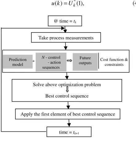
The main idea of receding horizon control is to use a model of the plant to predict the future evolution of the system. Based on this prediction, at each step k, the controller select a best sequence of control inputs by solving an optimization problem, which minimizes the tracking error, and in the meanwhile satisfies the active system constraints. Once the best sequence is obtained, only the first element of the sequence is actually applied to the plant. At next time step k+1, this procedure is repeated.

Consider the following optimal control problem

, || ) ( || || ) (

|| 2

1

2

min

e

N k

k i

s U

u

u i u x

i x

J

=

∑

+ − − + − =

∈

β

, ) (

)), ( ), ( ( ) | 1 (

, ) ( that such

max

min u k u

u

k u k x f k k x

x N k

x e

≤ ≤

= +

= +

(3)

where (xe, ue) is an equilibrium pair. (Definition 1 – Equilibrium pair: A vector x_e∈Rnand input ue∈S are said to be a equilibrium pair for system (1) if

e e

e u x

x

f( , )= , for ∀t>0.) N is the prediction horizon,

λ is a vector representing the relative importance (preference) of each variable in the cost function, and β is a vector penalizing control effort which aims to prohibiting frequent switching control. x(k) and u(k) are subject to the constraints (3). Assume for the current time instant k, the optimal solution U_k* = {u*(k),

) 1 (

., . . ), 1

( *

* _{+ + −}

N k u k

u } exists. According to the

receding horizon philosophy, the applied control action is set

), 1 ( ) (k U_k*

u = (4)

Figure 1. RHC using finite discrete inputs – FIRHC law

while the subsequent optimal inputs in U*_kare disregarded. At next step, this whole optimization procedure is repeated. The control law (2) - (4) is referred as the finite-input receding horizon control (FIRHC) law. Figure 1 shows this general idea of this control law.

Theorem 1: Let (xe,ue) be an equilibrium pair

2

. Providing the optimization problem (2) is feasible and is solved at each step, the FIRHC controller (2) – (4) stabilizes the system.

Proof: The proof follows from Lyapunov arguments.

Let U*_kbe the optimal control sequence at time instant k

in which Uk* = { ( ), ( 1),..., ( 1)

* *

* _{+ + −}

N k u k

u k

u } and N

is a pre-specified forward horizon. And let U~be a control sequence {u*(k+1),u*(k+2),…,u*(k+N−1),u_e}.

Consider that Uk*is such a control sequence that leads to

e

x , then U~is feasible at time k+1. Hence,

≤ +1) (k

Jopt JU~(k+1)

||, ) ( || || ) ( || ) 1

( _{e e}

opt k x k x u k u

J + − − − −

= (5)

and thus J_opt(k)is decreasing. J_opt(k)is also lower-bounded by 0. Therefore, the theorem is proved.

Remark 1: The terminal equality constraint in (3) is

added to ensure the stability of RHC approaches. The similar way to ensure the stability has been studied in the other linear and nonlinear RHC cases [5, 6]. With this constraint, the state is atx_e at the end of the finite horizon and therefore the control action isue; consequently if

there are no disturbances and a perfect prediction model is used, the system stays at the equilibrium state.

Remark 2: However, the terminal constraint added

also gives rise to more computational burden, and generally leads to a restrictive operating region, e.g., a region near the equilibrium state. In this regard, the theorem is rather about local stability than global stability. As is normally the case, Theorem 1 gives the sufficient condition for the stability.

Remark 3: The theorem provided assumes the

feasibility to imply stability. The added equality constraint adds the difficulty to achieve the feasible solution. It is clear that short horizons are desirable from a computational point of view. However, long horizon is necessary, at least helpful, to achieve the feasible solutions to ensure stability and enhance the closed loop performance. At next, a general approach is proposed to aiming at reducing the computational cost for seeking the solution.

II. 2. Sorted Depth First Search Algorithm

Given the fact that the total number of control inputs is finite and the forward prediction horizon is finite, the number of candidate control sequences as the solution for the optimization problem mentioned above is finite as well. Therefore, to solve the problem can be cast as a search process. As shown in [9, 10,11], a general approach to solve the discrete input involved predictive control problem is to use exhaustive search method in which all the permutations of control inputs sequence over the prediction horizon are exhaustively searched. Since the corresponding number of permutations is the cardinality of the control set raised to a power of the number of prediction horizon. Such a proposed exhaustive search can rapidly become computationally prohibitive as the horizon is defined longer.

We propose a general algorithm to sufficiently improve the computational efficiency. The motivation is taking advantage of the fact that all cost values are positive that are summed up along the forward horizon. The basic idea is that, if a low control sequence cost is found at the early stage in the searching, then many subsequent candidate sequences can be cut off even before they reach at the end of the horizon, providing that @ time = tk

Solve above optimization problem

Best control sequence

Apply the first element of best control sequence

time = tk+1

Take process measurements

Prediction model

N - control

- action sequences

+ _outputs Future Cost function &

the predicted cost at the middle of sequence already exceeds that low cost value. As a result of “cut off”, all the following permutations of that sequence can be cut off as well. Therefore, a lot of unnecessary computations will be avoided.

To implement the idea, a notion of node is defined. A node is a vector that is composed of the states, control action, depth and accumulated cost. The search is starting from the rooting node (i.e., current state) and is going further and further until reaching the end of horizon (similar to depth first search [13]), while expanding the new nodes along the horizon using state equations. Particularly, all freshly expanded nodes at the same depth, named as peers, will be sorted first by the cost value and added to a last-in-first-out stack for later expansion. The node with the lowest cost value among the peers will be put to the last of stack, which means, the node with lower cost value will get expanded first. As such, once the first sequence cost is achieved (expectedly a mildly low value), this value is stored as “optimal cost” which can be updated till the end of search. From then on, only the node with smaller cost than “optimal cost” can be added to the stack. As the searching along a sequence reaches the end of horizon (i.e., depth first), the search backtracks, returning to the most recent (last) node it has not finished exploring in the stack. The searching process terminates until the stack becomes empty.

In the regular cases, the space complexity of this algorithm is much lower than the exhaustive search since it only stores those nodes that are useful and qualified to expand. The time complexity is proportional to the number of total nodes once added to the stack that has been sufficiently reduced by the sorting process as mentioned above. The algorithm is presented in Table 1. In Sections IV, simulation results are provided to demonstrate the efficiency of the algorithm.

III SYSTEM DESCRIPTION OF A PNEUMATIC HOPPING ROBOT

III.1 Description for the Hopping Motion

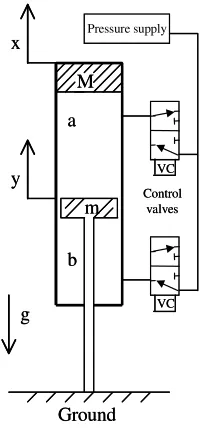
This work considers a vertical, gravity influenced pneumatic piston carrying an inertial load, serving as a hopping robot, as shown in Figure 2. The system contains two control inputs in the form of on/off three way valves that influence the mass flow into or out of each chamber a and b.

The kinetic and potential energy terms for a leakless, adiabatic (no heat losses), frictionless piston-mass system while in contact with the ground are given as [4]:

Mgx x A P P

P V P P

P V P x M E

x PEr

r atm x

PEb atm

b b b x

PEa atm

a a a x KE

+ + ⎥ ⎥ ⎥

⎦ ⎤

⎢ ⎢ ⎢

⎣ ⎡

− ⎟⎟⎠ ⎞ ⎜⎜⎝ ⎛ − + ⎥ ⎥ ⎥

⎦ ⎤

⎢ ⎢ ⎢

⎣ ⎡

− ⎟⎟⎠ ⎞ ⎜⎜⎝ ⎛ − + =

− −

43 42 1 4 4

4 3

4 4

4 2

1 4 4 4

4 3

4 4 4

4 2

1 3 2 1 &

& ()

) (

1

) (

1

) (

2 ₁

1 1 1

2

1 γγ γγ

γ γ

(6)

TABLE 1. SORTED DEPTH FIRST SEARCH ALGORITHM ---

Struct node {states, mode, depth, cost}; Stack node_array, temp_node_array; Struct node current_node, new_node;

Array path, best_path; Const horizon, mode_no; Var mode, best_cost;

best_cost =

+

∞

; //assign the initial cost

Push (node_array, root_node); //initialize with the current state

WHILE node_array ~= empty

current_node := Pop(node_array); //remove last element of stack path(current_node.depth):=current_node.mode; //remember current

path

IF current_node.cost < best_cost THEN FOR i =1: mode_no

SWITCH {mode} CASE(mode)

new_node := Compute(current_node, mode); //a function to generate a child node, depth++ ENDSWITCH

IF new_node.cost < best_cost && new_node.depth ~= horizon THEN

Push(temp_node_array, new_node); ENDIF

IF new_node.cost < best_cost && new_node.depth == horizon && Terminal_equality_check( ) == true THEN

best_cost := new_node.cost; //update best_cost path(new_node.depth) := mode;

best_path := path; //update the best path so far ENDIF

ENDFOR

IF temp_node_list is not empty THEN

Sort_descending(temp_node_list); //sort the nodes by costs Push(node_array, temp_node_list);

//push in last the node with lowest cost ENDIF

ENDIF ENDWHILE

u* := best_path(1); //the first element of the best path is the one wanted

--- where V_a,b represents the volume of chamber a or b, and

b a

r A A

A = − represents the cross sectional area of the piston rod. The potential energy of each chamber of the actuator is derived using standard thermodynamic relationships as the ability of the pressure in the chamber,

a

P orPb, to do work adiabatically with respect to an

M m Ground y x g a b Pressure supply VC VC Control valves M m Ground y x g a b Pressure supply VC VC Control valves

Figure 2. Schematic of a pneumatic robot

Ideally (no energetic loss), the motion equations can be obtained by settingE&=0:

Mg A P A P A P x

M&&= a a− b b − atm r− (7)

mg F A P A P A P y

m&&= b b− a a + atm r + ground− (8)

Expressions for the time rates of change of the pressures can be derived from the following constitutive relations for the rate of internal energy storage U& , rate of heat input Q&, enthalpy rate H& , and work rate W& , of each control volume associated with side a and side b:

U& =Q&+H& −W& (9)

1 − + = γ V P V P

U& & & (10)

flow pT

c m

H& = & (11)

V P

W& = & ₍₁₂₎

These result in the following for Q& =0 (adiabatic):

a a a a a flow a V V P m V RT

P& =γ & −γ & (13)

b b b b b flow b V V P m V RT

P& =γ & −γ & (14)

The standard equations for the mass flow through the orifice are given by Ben-Dov and Salcudean [14]:

. ) ( 1 ) ( ) flow chocked ( , otherwise , then , 528 . 0 If / ) 1 ( / 1 1 , 1 , k k u d k u d u v f b a u v f b a u d P P P P T P C A C m T P C A C m P P − ⋅ ⋅ − = = ≤ (15) where A_vis orifice area, C_f is discharge coefficient, T is

temperature of flow, P_u and P_dare, respectively, upstream and downstream pressure.

A hopping cycle can be defined as shown in Figure 3. The corresponding moments and periods are defined [4]:

0

0 =

t defines the starting point of a full hopping cycle (x = 0).

1

t defines the lift-up moment of the foot (y = 0).

0 1

1 t t

T = − is defined as the launch period.

2

T is defined as the compression period (x≤0).

air

T is defined as the flight time.

3

T is defined as the recovery period.

hop

T is defined as the full hopping period.

0

Time 1

T T2

0

t t₁

air

T T3

0

x

y

1

T T2

0

t t₁

air

T T3

1

T T2

0

t t₁

air

T T3

Di

splacem

en

t

Figure 3. A hopping cycle

As defined above, the hopping cycle can be analyzed according to the following decomposition,

2 3

1 T T T

T

T_hop≅ + + _air + (16)

where Thop and Tair are to be specified, and T3≅T1.

III.2 Derivation of the Desired Total Conservative Energy

It should be noted that the conservative energy storage expression of Equation (6) is valid only when the contact with ground is maintained. It is sufficient to control the energy storage during contact only. Therefore, the proposed control strategy is to switch the valves only in the contact period to regulate the total energy around the desired point (thus the desired hopping motion can be achieved), and seal off the valves in flight. A critical step is to achieve the desired conservative energy value given the pre-specified motion index - total hopping period Thop

and flight time Tair.

The procedure to derive the desired total conservative energy of the system to support the desired Thop and Tair is

summarized below. For the limit of space, only critical equations are listed. For more details, find [4].

Given Thop and Tair, compute T2 by solving the

following equation: 2 2 2 2 2 ) / ( ) ( 8 ) ( 8 arcsin 2 T T gT T M g m M g m M T T _air air

hop _⎟⎟+ +

Compute x(t₁)andx&(t₁) using the following equation and results from (17)

2 2 1

) / (

) ( ) (

T M

g m M t

x

π

⋅ +

≅ (18)

2 ) (t₁ T g

x& = air (19)

Utilizing the above results and substituting into Equation (6), compute the desired total conservative energy of the system:

) ( ) ( ))

( ( )) ( ( )

( 1 1 1 1

2 1 2

1_{Mxt PEaxt PEbxt P A xt Mgxt}

Ed = & + + + atm r +

(20) Since it is known that the energy of the system when leaving and touching with the ground is identical (except for losses), regulating the system to maintain the desired total energy (ideally, hopping with constant energy) in contact will result in the desired hopping motion.

IV SIMULATION EXPERIMENTS

IV.1Experiment 1

A simulation of a controlled pneumatic hopping robot involving frictional losses is presented as below. The hopping system was modeled as the following with added friction terms of equations (7) and (8):

Mx&&=P_aA_a−P_bA_b−P_atmA_r−Mg−b(x&−y&) (21) ) (y x b mg F

A P A P A P y

m&&= _{b b}− _{a a}+ _{atm r}+ _ground− − &−& (22)

with M = 0.54 kg and m = 0.05 kg, and viscous friction effects representing the sliding piston and rod seals modeled by b = 2 Ns/m. The pressure dynamics were modeled as equations (13) and (14). The ground model was approximated as a very stiff spring and damping to represent losses upon collision,

, 0 if , <

− −

= k y b y y

F_{ground ground ground}& (23)

where kground=

6

10 0 .

1 × N/m and bground = 1000 N.sec/m.

The procedure listed in Section III.2 is used to derive the desired total conservative energy given a pre-specified motion index. For example, given Thop = 0.4s

and T_air= 0.2s, T₂can be pre-computed by solving equation (17) using a nonlinear solver. As a result, T₂ = 0.161s. Following the procedure, the desired energy Ed = 11.44. In this case, the control of side a is to compensate mostly for leakage, the mass flow rate must be greater than some number when the chamber is under pressurized, the following on/off control law will be used for side a while in contact with the ground: Charge

chamber a if

γ

⎟⎟⎠ ⎞ ⎜⎜⎝

⎛

+ <

x A V

V P P

a mida

mida a

a 0 andy≤0, where

0

a

P and V_midaare respectively static equilibrium pressure and volume of chamber a. The mass flow into chamber b is used to maintain the energy. Supply pressure Ps = 80 psi. Here only the terminal equality constraint on total energy is enforced. As the desired velocity reference used

is approximately ideal with no friction and other losses, it may make the problem intractable to require a terminal constraint on the velocity term. The other setting for (2) is that λ₁=1,λ₂ =0.1, andβ =10. Horizon N is set to be 6. For this problem, Equation (2) and (3) becomes

. 01 . 0 ) ( 01 . 0

, ) 6 (

), 15 ( and ), 14 ( ), 13 ( ), 8 ( ), 7 ( ), 6 ( . Eqn to subject is ) 1 ( s.t.

) ( 10 )) 1 ( ) 1 ( ( 1 . 0 ) ) 1 ( ( min

5

2 2

2

≤ ≤ −

= + +

+ + − + + − + =

∑

+

∈

i u

E k E

i E

i u i

x i x E

i E J

d k

k

d d

U

u & &

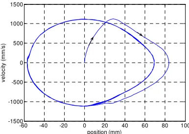
(24) Fig. 4 – 8 show the simulation results of the hopping robot for T_air = 0.4s and T_air = 0.2s. Fig.4 shows the hopping behavior. As a result, the average T_hop

≅

0.39

and T_air ≅ 0.19s that means the motion is well controlled. It is better than previous work [4] where Thop

≅ 0.39 and average T_air

≅

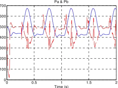
0.18s. Fig.5 shows that the system is stabilized in a desired circle. Fig.6 displays the pressures’ time evolution. Fig.7 and 8 give close looks on the total energy evolution and mass flow b during a compression period. They demonstrate under the unpredicted friction, the proposed controller effectively regulates system energy around the desired point.

0 0.5 1 1.5 2

-60 -40 -20 0 20 40 60 80 100

x & y

Time (s)

Figure 4. Displacements of hopping robot, dotted: y

-60 -40 -20 0 20 40 60 80 100 -1500

-1000 -500 0 500 1000 1500

position (mm)

ve

lo

ci

ty (

mm/

s)

0 0.5 1 1.5 2 0

100 200 300 400 500 600 700

Pa & Pb

Time (s)

Figure 6: Pressure of Chamber a and b, dotted: Chamber b

0.7 0.75 0.8 0.85

1.115 1.12 1.125 1.13 1.135 1.14 1.145 1.15

x 107 Current Energy

Time (s)

Figure 7: Energy regulation in a compression period (T2 = 0.165),

dotted: desired energy

0.7 0.75 0.8 0.85

-4 -3 -2 -1 0 1 2 3 4

x 10-3 mass flow b

Time (s)

Figure 8: Mass flow into Chamber b in a compression period

Several sets of 2-second-simulations are conducted to check on the efficiency of the proposed sDFS method. Table 2 displays the results for cases of horizon = 5, 6, 7, and 8. Note that Point A represents nodes visited at a step in ES, Point B represents nodes visited at a step in sDFS, (max/min), and Point C denotes the total time of sDFS /total time of ES (%).

The final column (Point C) is achieved by executing two methods on the same experiment settings of the hopping system. It is apparent that sDFS always has fewer nodes to visit by comparing the elements between Point B column and Point A column. And as horizon becomes longer, the sDFS has better and better performance compared to the exhaustive search (ES).

TABLE 2: EXHAUSTIVE SEARCH AND SORTED DEPTH FIRST SEARCH FOR

EXPERIMENT 1

Point A Point B Point C

5 363 363/15 7.0%

6 1,092 1,044/18 4.1%

7 3,279 2,208/21 2.3%

8 9,840 4,380/24 1.1%

IV.2 Experiment 2

To further illustrate the efficiency of sDFS algorithm when it is applied to a relatively large multi-mode system, a three tank fluid system example is introduced. The fluid system consists of three identical tanks, connected in a series configuration. Transfer of fluid through different paths is made possible by on/off control of a set of solenoid operated valves in the system. The fluid flow into and out of each tank is controlled by three valves: (i) an inflow, (ii) an outflow, and (iii) a bypass valve. Three additional valves in the system provide further control of the fluid flow in the system. The fluid level in each tank is measured. This system has been successfully realized online using the similar control strategy [10]. Intending to simplify the computations, the total operation modes that can be up to 27 = 128 have been reduced to 17 in which the controllability is well maintained. The prediction horizon still has to be limited to no larger than four since only exhausted search was used then to derive the best control solution at each step.

Given a particular mode of system operation – The second tank is filling at low speed and the first tank transferring fluid to the third tank. For this mode, u = {VFill1 = 0, VFill2 =1, Vtrans1 = 1, Vtrans2 = 0, Vtrans3 = 1, pump = low}T, and Flowlow is the corresponding constant flow provided by the pump with low speed. The discrete time state equations for this mode are

)) ( / ) ( ) ( / )) ( ) ( (( ) ( ) 1 (

) / ( ) ( ) 1 (

))) ( / )) ( ) ( (( ) ( ) 1 (

3 3 2 3 1 3

3

2 2

1 1 3 1

1

k k h k k h k h t k h k h

A Flow t k h k h

k k h k h t k h k h

s low s s

τ

τ

τ

− −

+ = +

+ = +

− +

= +

(25)

where sampling timet_s =2s,Ais cross section area of

tanks, and

τ

₁

(

k

),

τ

₂

(

k

),

and

τ

₃

(

k

)

are state-dependent time constants at kth instant. For the limit of space, refer to [10] for more details on the parameters.

the sDFS algorithm turns a typically heavy computation into a much more manageable task.

TABLE 3: EXHAUSTIVE SEARCH AND SORTED DEPTH FIRST SEARCH FOR

EXPERIMENT 2

V. CONCLUSIONS

In this paper, a finite-input receding horizon controller is presented to deal with a kind of switching control systems where only a finite number of discrete-valued controls are available. The controller design is motivated by the need of motion control of a pneumatic hopping robot using on/off solenoid valves. The pneumatic motion control problem is studied and recast as an energy regulation problem. A desired total conservative energy is computed and serves as an objective in the control scheme. Simulation results demonstrate the effectiveness of the proposed (FIRHC) controller. Stability analysis is discussed. The terminal equality constraint is added to ensure the stability, but it leads to severe restriction of the operation region of the system. More effective stability condition needs to be developed.

In addition to the controller design, this paper develops an efficient approach, sorted depth first search (sDFS), to seek solutions of the optimization problem in the proposed controller. The algorithm takes advantage of the fact of cost always being positive and expands first the nodes with lower cost to avoid unnecessary computation. It has been effectively applied for the motion control system, and for the further demonstration it is used for a three tank system that has a relatively large amount of operation modes. The simulation results show that compared to exhaustive search, the previously generally used method in the same kind of problem, sDFS achieves much better efficiency in both cases.

REFERENCES

[1] M. Raibert, Legged Robots that Balance, MIT Press,

Cambridge, MA, 1986.

[2] M. Binnard, Design of a Small Pneumatic Walking Robot, master’s thesis, MIT, Cambridge, MA, 1995.

[3] N. M’sirdi, N. Manamani, and N. Nadjar-Gauthier, “Methodology based on CLC for Control of Fast Legged Robots,” Proceedings of the 1998 IEEE/RSJ International Conference on Intelligent Robotics and Systems, Victoria, B.C., Canada, pp. 71-76, 1998.

[4] Y. Zhu, and E. Barth, “An Energetic control methodology for pneumatic hopping robot,” submitted to IEEE/ASME Transactions on Mechatronics, 2006.

[5] E. Camacho and C. Bordons. Model Predictive Control, Springer, London, 1999.

[6] J. Maciejowski, Predictive Control with Constraints, Prentice Hall, London, 2002.

[7] S. J. Qin and T. A. Badgwell. “An overview of industrial model predictive control technology,” in J. C. Kantor, C. E. Garcia, & B. Carnahan (Eds.), Chemical process control—V, Fifth international conference on chemical process control CACHE and AICHE, pp. 232–256, 1997. [8] S. J. Qin and T. A. Badgwell. “An overview of nonlinear

model predictive control applications.” in F. Algower, & A. Zheng (Eds.), Nonlinear model predictive control workshop—assessment and future directions, Ascona, Switzerland, 2000.

[9] T. Tsang, and D. Clarke, “Generalized Predictive Control With Input Constraints,” IEEE Proceedings—Control Theory and Applications, 135(6), pp. 451–460, 1988. [10] J. Wu, S. Abdelwahed, and G. Biswas, “A Hybrid Control

System Design and Implementation for a Three Tank Test-bed”, in Proc. IEEE Conference on Control Applications, pp. 645 – 650, Toronto, Canada, September 2005.

[11] S. Abdelwahed, J. Wu, G. Biswas, and E. Manders, “Online Fault Adaptive Control for Efficient Resource Management in Advanced Life Support System,”

Habitation – International Journal for Human Support Research, 10(2): 105 – 115, 2005.

[12] B. Shields, E. Barth, and M. Goldfarb, “Predictive Control for Time Delayed Switching Control Systems,” Journal of Dynamic Systems, Measurement, and Control, vol. 128, 999-1004, Dec. 2006.

[13] T. Cormen, C. Leiserson, R. Rivest, and C. Stein,

Introduction to Algorithms, Second Edition. pp.540–549, MIT Press and McGraw-Hill, 2001.

[14] D. Ben-Dov, and S. Salcudean, ‘‘A Force-Controlled Pneumatic Actuator,’’ IEEE Trans. Robotic Automation, vol. 11, No. 6, pp. 906–911, 1995.

Jian Wu was born in Harbin, China. He received a Master of Engineering degree in control theory and applications from Harbin Institute of Technology, Harbin, China in 1997, and a Master of Science degree in Electrical Engineering from Vanderbilt University, Nashville, TN in 2007.

He is currently a controls analyst with Omron Oilfield and Marine in Houston, TX. His major research interests involve AC/DC drive systems modeling, control and simulation, digital control techniques of nonlinear systems, and model predictive control theory and applications.

Sherif Abdelwahed is an Assistant Professor with Electrical and Computer Engineering Department at Mississippi State University. He received his Ph.D. degree in Electrical and Computer Engineering from the University of Toronto, Canada, in 2002. From 2000 to 2001, he was a research scientist at Rockwell Scientific Company. From 2002 to 2007 he worked as a research assistant professor with the Institute for Software Integrated Systems at Vanderbilt University. His main research interests include model-based design and analysis of self-managing computation systems, modeling and analysis of distributed real-time systems, automated verification, fault diagnosis techniques, and model-integrated computing. He has published over 70 publications. He is a senior member of the IEEE and member of Sigma Xi.

Horizon Point A Point B Point C

3 5,219 2,516/595 16%

4 88,740 13,396/1,377 3.1%

5 1,508,597 44,608/3,009 0.6%