Clustering in Wireless Multimedia Sensor Networks Using Spectral Graph Partitioning

Clustering in Wireless Multimedia Sensor Networks

Using Spectral Graph Partitioning

Pushpender Kumar, Narottam Chand

Department of Computer Science and Engineering, National Institute of Technology, Hamirpur, India Email: [email protected], [email protected]

Received January 11, 2013; revised February 13, 2013; accepted March 11,2013

ABSTRACT

Wireless multimedia sensor network (WMSN) consists of sensors that can monitor multimedia data from its sur- rounding, such as capturing image, video and audio. To transmit multimedia information, large energy is required which decreases the lifetime of the network. In this paper we present a clustering approach based on spectral graph par- titioning (SGP) for WMSN that increases the lifetime of the network. The efficient strategies for cluster head selection and rotation are also proposed.

Keywords: Wireless Multimedia Sensor Network; Eigenvector; Spectral Graph Partitioning

1. Introduction

Wireless sensor network (WSN) consists of hundreds or even thousands of sensor nodes that are powered by small irreplaceable batteries. The sensors, which are ran- domly deployed in an environment, should collect data from their surrounding, process the data and finally send it to the sink through multi hops [1]. There are many ap- plications where sensor nodes are deployed onto roads, walls or unreachable place and they sense a variety of physical phenomena such as traffic on the road, tem-perature, pressure or detect forest fires to aid rapid emer- gency response. WSN has limited resources such as less communication bandwidth, limited energy supply, less storage and less computing power [2].

Wireless multimedia sensor network (WMSN) has been possible due to the production of cheap CMOS (Complementary Metal Oxide Semiconductor) camera and microphone sensors which can acquire multimedia information. WMSN consists of camera sensors as well as scalar sensors. Camera sensors can retrieve much rich- er information in the form of images or videos and hence provide more detailed and interesting data about the en-vironment [3]. Scalar sensors can retrieve the scalar phe- nomena like temperature, pressure, humidity, or location of objects [4]. Camera sensors may generate very differ- ent views of the same object if they are taken from dif- ferent viewpoints [5].

Sensor nodes (SN) are deployed in remote and hostile environment, so it is difficult to replace the batteries. They are densely deployed to monitor the physical envi- ronment. In case of WMSN, the neighboring sensors

would produce similar data and transmit such data to the sink. During this transmission of data, a large amount of energy is consumed. To reduce the energy consumption some kind of grouping of sensor nodes can be done to form clusters. Inside every cluster, one node acts as clus- ter head (CH). Cluster head is responsible for communi- cation with other cluster heads. Cluster head collects data from all the nodes within its cluster, aggregates this in- formation and then transmits to the sink through other CHs using multi hop communication [2]. Figure 1 shows the clustering of nodes in a general WSN. In WMSN, the volume of multimedia data to be transmitted is very large, therefore, more energy consumption occurs during com- munication [6].

In this paper, we propose a clustering and cluster head selection approach. Spectral graph partitioning (SGP) tech- nique based upon eigenvalues proposed by Fiedler has been utilized for WMSN [11]. SGP method has been used in many applications such as image segmentation, social networks, etc. [2].

The spectral graph partitioning (SGP) algorithm is based on second highest eigenvalues of particular graph. The second smallest eigenvalue of the Laplacian matrix corresponding to different eigenvectors, is used to parti-tion the graph into two parts. Within a cluster, a node with highest eigenvalue is selected as cluster head. In case of WMSN, large volume of sensed data is generated, therefore, such clustering can be utilized to reduce the volume and number of data transmissions through data aggregation. In this paper, we have shown formation of clusters and CH selection using SGP for given WMSN.

Base Station/Sink

Cluster 1

Cluster 2

Cluster 3 Cluster Head Sensor Node

Figure 1. Clustering of SNs in WSN.

reviews the related work. General SGP strategy for clus-tering has been presented in Section 3. Section 4 de- scribes the use of SGP for WMSN. Section 5 concludes the paper.

2. Related Work

Clustering in WSN is a process in which set of sensor nodes are loosely connected and work together. All the nodes in the cluster elect one cluster head which is re-sponsible for data aggregation and data transmission and maintaining connectivity between other cluster heads.

Brahim Elbhiri et al. [6] suggested spectral classifica- tion based on near optimal clustering in wireless sensor networks (SCNOPC-WSN) algorithm. This algorithm deals with the clustering problem in WSN. Energy aware adaptive clustering protocol is used for the bi-partitioning spectral classification and it guarantees robust clustering. SCNOPC-WSN also deals with the optimization of the energy dissipated in the network.

M. Chatterjee et al. [7] suggested the weighted clus- tering algorithm (WCA) for ad hoc networks. WCA uses the on-demand clustering algorithm in multi hop radio networks. WCA elects the head nodes on the basis of neighboring nodes and their sending capabilities.

Banerjee and Khuller [8] suggested hierarchical clus-tering algorithm based on geometric properties of the wireless network. Generic graph algorithms developed for arbitrary graphs would not exploit the rich geometric information present in wireless network. Clustering prob- lem in a graph is theoretical framework and presents an efficient distributed solution.

Adaptive Clustering Protocol is proposed by A. Garg and M. Hanmandlu [9]. It divides the network into sev- eral systematized hexangular and chooses the closest node to each hexangular as the head node for it. The nodes with the maximum amount of residual energy is

selected as a cluster head.

Lu Dian et al. [10] proposed a clustering based spec-trum allocation scheme for efficient specspec-trum allocation in cognitive radio networks. Spectral graph partitioning theory is used to divide a graph into clusters so that spec-trum allocation is executed in parallel.

3. Cluster Handling Using SGP

Spectral graph partitioning technique uses information obtained from the eigenvalues and eigenvectors of their adjacency matrices for partitioning of graphs. The meth-ods are called spectral, because they make use of the spectrum of the adjacency matrix of the data to cluster the points [11]. Spectral methods are widely used to compute graph separation. Spectral graph partitioning is a powerful technique in data analysis that has found in-creasing support and applications in many areas such as image segmentation and social network analysis. SGP divides the graph into two disjoint groups, based on ei-genvectors corresponding to the second smallest eigen-value of the Laplacian matrix [10].





Let G V E, is an undirected graph where V repre-sents the set of vertices (nodes) and E represents the set of edges connecting these vertices. Each vertex is identi-fied by an index i





N N

1 edge weight between node and node 0 otherwise.

ij

i j

A a _{ }   

N N The edge between node i and node j is represented by eij. The graph can be

rep-resented as an adjacency matrix. The adjacency matrix A of graph G having N nodes is the _{matrix where} the non-diagonal entry aij is the number of edges from

node i to node j, and the diagonal entry aii is the number

of loops at node i. The adjacency matrix is symmetric for undirected graphs [12].

The adjacency matrix A is defined as

We also define degree matrix D for graph G. The de-gree matrix is a diagonal matrix which contains informa-tion about the degree of each node. It is used together with the adjacency matrix to construct the Laplacian ma-trix of a graph. The degree mama-trix D for G is a 

square matrix and is defined as

total weight of edges incident to node deg

0.

ij

i D_ _{ }

 

N N

L D A

The Laplacian matrix is the combination of adjacency matrix and the degree matrix. The Laplacian matrix of the graph G having N vertices is square matrix and is represented as

 

 

1 if and d

1

, if node and node deg deg

0 otherwise

j

i j

i j

i j i

 _{ }         eg 0

are adjacentj



The eigenvalues of matrix are denoted by _i, such that

1, 2, ,

i  N ₁₂ _n. ,

X X

 Laplacian ma-trix has the property   

  

 

where X is the ei-genvector of the matrix and λ is the eigenvalue of the matrix . Laplacian matrix plays important role in spectral graph theory. λ1 represents the number of

sub-graphs in the network. The second smallest eigenvalue λ2

is referred to the algebraic connectivity and its corre-sponding eigenvector is usually referred to as the Fiedler Vector [13].



We choose the eigenvector values corresponding to the second smallest eigenvalue λ2. Second highest eigenvalue

2

 divides the graph into two subgraphs. G is divided into two subgraphs G+ _{and G}−_{, where G}+ _{and G}− _{are the}

set of vertices related to the new subgraphs. G+ _contains

nodes corresponding to positive eigenvalues and G−

con-tains nodes corresponding to negative eigenvalues. The set of vertices is defined by N_N_N such that

N_N__{, where N G, N}_G _{and N}_{ G}

 

. Based on the above concept, in next section we have proposed a new approach to partition the WMSN into the clusters.

4. Cluster Formation in WMSN

Here we apply the SGP technique to partition the net-work. SGP has many advantages as compared to other clustering algorithms. While clustering, it results in few links to other clusters but intra-cluster communication is high. Each node is at one hop distance from other node within the cluster. If the graph is to be partitioned into more than two subgraphs, apply SGP technique recur-sively. High intra-cluster similarity between the nodes makes SGP technique a better option for multimedia data clustering.

In our proposed method, clustering of WMSN has been done by applying Spectral Graph Partitioning tech-nique [10] recursively. Each node sends short message to sink which contains the location information of the node. On the basis of this information, the sink constructs the adjacency matrix and degree matrix and then constructs the Laplacian matrix. The eigenvector corresponding to second smallest eigenvalue (called Fiedler Vector) is used to partition the WMSN. The location of each node may be found by GPS (Global Positioning System) or any other localization method [14,15].

4.1. Steps for Clustering

 Construct a graph G for the given sensor network.

 Construct the normalized Laplacian matrix, defined as

1 if and deg 0

1

, if node and node are adjacent deg deg

0 otherwise

j

i j

i j

i j i j

 _{ }        

where degiis the degree of node i.

 Form the Laplacian matrix  of the graph. Compute the eigenvalues and eigenvector of Laplacian matrix.  Select the second smallest eigenvalue λ2 of Laplacian

matrix .

 Choose eigenvector value corresponding to the ei-genvalue λ2.

 Divide the graph G into two sub-graphs G+ _{and G}−_,

where G+ _{contains nodes corresponding to positive}

eigenvalues and G− _{contains nodes corresponding to}

negative eigenvalues.

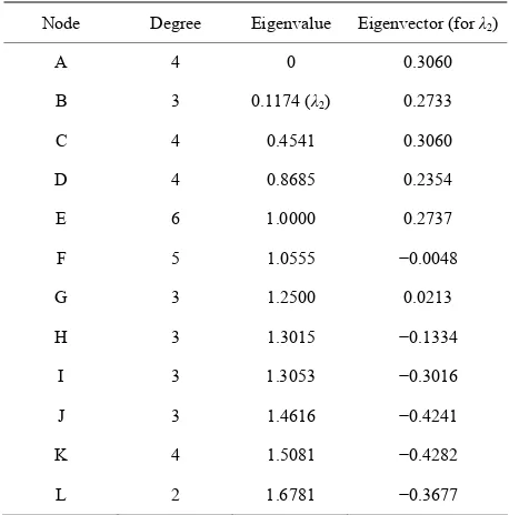
After the first iteration of above algorithm, the whole network is divided into two clusters based on the eigen-values of the nodes. Table 1 shows the two partitions/ clusters for a given graph shown in Figure 2. After first iteration cluster 1 contains all the nodes with positive eigenvector values and another cluster 2 contains nodes having negative eigenvector values. Cluster 1 has six nodes A, B, C, D, E, and G with positive values of ei-genvector. Cluster 2 has six nodes F, H, I, J, K and L that have negative eigenvector values. These clusters are listed in Table 2.

Only two clusters are formed in first iteration as shown in Figure 3. The larger cluster can be further divided into

Table 1. Eigenvector table and clustering of given network.

Node Degree Eigenvalue Eigenvector (for λ2)

A 4 0 0.3060

B 3 0.1174 (λ2) 0.2733

C 4 0.4541 0.3060

D 4 0.8685 0.2354

E 6 1.0000 0.2737

F 5 1.0555 −0.0048

G 3 1.2500 0.0213

H 3 1.3015 −0.1334

I 3 1.3053 −0.3016

J 3 1.4616 −0.4241

K 4 1.5081 −0.4282

Figure 2. Given graph.

Figure 3. Clustering after first iteration.

Table 2. Initial cluster for the network. two different clusters by applying the algorithm

recur-sively. This process continues until maximum intra-node

distance within a cluster is less than Cluster Number Nodes Eigenvalue Cluster 1 A, B, C, D, E, G Positive

Cluster 2 F, H, I, J, K, L Negative 2 2 ,

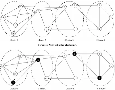
R where R is the transmission rang of the sensor node. When intra- node distance within a cluster is less than R 2 2 ,two nodes in neighboring clusters can communicate in one hop. After applying the algorithm recursively, the given network is divided into four clusters as shown in Figure 4.

Table 3. Final clusters for the network.

Cluster Number Nodes

Cluster 1 A, B, C, D

Cluster 2 E, G

Cluster 3 F, H, I

Cluster 4 J, K, L It has been observed that both the clusters have higher

intra-node distance than R 2 2 , so apply the algo-rithm to both the clusters. After applying the algoalgo-rithm cluster 1 is portioned into two different clusters. This algorithm is also applied to cluster 2 of Figure 3.

Thus the whole network is divided into four clusters as shown in Figure 4. Table 3 shows different nodes

pre-sent in the each cluster. _{represents the eigenvector values of the cluster and} Ta-ble 5 shows the elected cluster heads in different clusters on the basis of eigenvector values. Therefore, we com-pare the eigenvector values of the cluster and choose the least eigenvector node as a cluster head, i.e.

4.2. Cluster Head Election

The clustering algorithm divides the whole network into clusters. The next step is election of cluster head for each cluster. As per the property of SGP, the least eigenvector value of node signifies that the node is well connected to the other nodes within the cluster as well as it is con-nected to cluster [13].

Cluster Head Least Eigenvector

Figure 5 shows the elected cluster heads for different clusters.

Cluster head rotation must take place when residual energy

For initial cluster head election, we chose the least

Figure 4. Network after clustering.

Figure 5. Elected cluster heads for different clusters.

Table 4. Clustering after second iteration.

Node Initial Cluster Eigenvalue Eigenvector _{(for λ}

2) Cluster

A 0 −0.2833

B 0.7353 (λ2) −0.1808

C 1.0000 −0.2833

D 1.2500 −0.1808 Cluster 1

E 1.4332 0.4418

G

C L U S T E R 1

1.5815 0.7572 Cluster 2

F 0 −0.5862

H 0.5124 (λ2) −0.4808

I 0.9293 −0.1103 Cluster 3

J 1.2611 0.4113

K 1.4616 0.1660

L

C L U S T E R 2

1.8356 0.4648 Cluster 4

threshold value th . The present cluster head declares

the election process by sending a message that contains its Eres to all the cluster members. The cluster members

whose residual energy is greater than Eres responds to this

Table 5. Elected cluster heads.

Cluster Number Eigenvector Cluster Head

Cluster 1 0.1808 B

Cluster 2 0.4418 E

Cluster 3 0.1103 I

Cluster 4 0.1660 K

message by sending the residual energy to the cluster head.

The new cluster head is elected based upon CH Can-didacy Factor

 

 

res i

i i

E CF

D 

i

E

where res is the residual energy of node i, Di is the

distance between node i and current cluster head. If











 



are the location coordinates of current cluster head and node i, respectably, then

2 2

i ch i ch i

D  x x  y y

5. Conclusion

This paper has proposes an approach to deal with the clustering problem in a given wireless multimedia sensor network. The proposed algorithm partitions the given WMSN into clusters such that nodes in a cluster are highly correlated and intra-cluster association is mini-mized. In WMSN where nearby nodes have common interest in terms of sensing, our proposed algorithm is more suitable. Further we define the algorithm for cluster head election and rotation. The given strategy can be used in WMSN to prolong the network lifetime.

REFERENCES

[1] F. Akyldiz, W. Su, Y. Sankarasubramaniam and E. Cay- irci, “Wireless Sensor Networks: A Survey,” Computer Networks, Vol. 38, No. 4, 2002, pp. 393-422.

doi:10.1016/S1389-1286(01)00302-4

[2] B. Elbhiri, S. El Fkihi, R. Saadane and D. Aboutajdine, “Clustering in Wireless Sensor Network Based on Near Optimal Bi-Partitions,” EURO-NF Conference on Next Generation Internet (NGI), 2-4 June 2010, pp. 1-6. [3] Y. Wang and G. H. Cao, “On Full-View Coverage in Ca-

mera Sensor Networks,” IEEE International Conference on Computer Communications (INFOCOM), 10-15 April 2011, pp. 1781-1789.

[4] I. F. Akyildiz, T. Melodia and K. R. Chowdhury, “A Sur- vey on Wireless Multimedia Sensor Networks,” Com- puter Networks, Vol. 51, No. 4, 2007, pp. 921-960. doi:10.1016/j.comnet.2006.10.002

[5] A. Newell and K. Akkaya, “Self-Actuation of Camera Sensors for Redundant Data Elimination in Wireless Mul- timedia Sensor Networks,” IEEE International Confer-ence on Communication, 14-15 June 2009, pp. 1-5. [6] C. Intanagonwiwat, R. Govindan and D. Estrin, “Directed

Diffusion for Wireless Sensor Network,” ACM/IEEE Tran- sactions on Networking (TON), Vol. 11, No. 1, 2003, pp. 2-16. doi:10.1109/TNET.2002.808417

[7] M. Chatterjee, S. K. Das and D. Turgut, “WCA: A Weighted Clustering Algorithm for Mobile Ad Hoc Net-works,” Journal of Cluster Computing, Vol. 5, No. 2, 2002, pp. 193-204. doi:10.1023/A:1013941929408 [8] S. Banerjee and S. Khuller, “A Clustering Scheme for

Hierarchical Control in Multi-Hop Wireless Networks,” IEEE International Conference on Computer Communi- cations (INFOCOM), 16-21 July 2001, pp. 1028-1037. [9] A. Garg and M. Hanmandlu, “An Energy-Aware Adap-

tive Clustering Protocol for Sensor Networks,” Interna-tional Conference on Intelligent Sensing and Information Processing (ICISIP), 2006, pp. 13-30.

[10] D. Lu, N. Jie and X.-X. Huang, “Clustering Based Spec- trum Allocation Scheme in Mobile Ad Hoc Networks,” Bulletin of Advanced Technology Research (BATR), Vol. 5, No. 12, 2011, pp. 37-41.

[11] B. Auffarth, “Spectral Graph Clustering,” Course Report. http://www-lehre.inf.uos.de/~bauffart/spectral.pdf [12] Adjacency Matrix Wikipedia.

http://en.wikipedia.org/wiki/Adjacency_matrix

[13] A. Bertrand and M. Moonen, “Distributed Computation of the Fiedler Vector with Application to Topology Infer- ence in Ad Hoc Networks,” Signal Processing, Vol. 93, No. 5, 2013, pp. 1106-1117.

[14] A. Savvides, C. Han and M. B. Srivastva, “Dynamic Fine- Grained Localization in Ad Hoc Networks of Sensors,” International Conference on Mobile Computing and Net- working (MOBICOM), 16-21 July 2001, pp. 166-179. doi:10.1145/381677.381693