DOI 10.1007/s13173-012-0077-3 W T I
Forgetting mechanisms for scalable collaborative filtering
João Vinagre·Alípio Mário Jorge
Received: 26 May 2011 / Accepted: 27 April 2012 / Published online: 17 May 2012 © The Brazilian Computer Society 2012
Abstract Collaborative filtering (CF) has been an impor-tant subject of research in the past few years. Many achieve-ments have been made in this field, however, many chal-lenges still need to be faced, mainly related to scalability and predictive ability. One important issue is how to deal with old and potentially obsolete data in order to avoid unnec-essary memory usage and processing time. Our proposal is to use forgetting mechanisms. In this paper, we present and evaluate the impact of two forgetting mechanisms—sliding windows and fading factors—in user-based and item-based CF algorithms with implicit binary ratings under a scenario of abrupt change. Our results suggest that forgetting mecha-nisms reduce time and space requirements, improving scala-bility, while not significantly affecting the predictive ability of the algorithms.
Keywords Collaborative filtering·Recommender systems·Forgetting·Data streams
1 Introduction
Collaborative filtering (CF) has been successfully used in a large number of applications, such as e-commerce
web-This is a revised and extended version of a previous paper that appeared at WTI 2010 (III International Workshop on Web and Text Intelligence) and has been recommended to JBCS.
J. Vinagre (
)·A.M. JorgeDCC–FCUP, Universidade do Porto, Porto, Portugal e-mail:[email protected]
A.M. Jorge
e-mail:[email protected] J. Vinagre·A.M. Jorge
LIAAD–INESC TEC, Porto, Portugal
sites [12] and on-line communities in a series of domains [9, 19, 21]. However, some challenges are still offered. Most of these systems deal with very large amounts of data and frequently suffer from scalability problems. CF systems should be able to efficiently process data on-line as it ar-rives, in order to keep the system up-to-date. This poses two problems:
– Scalability: as new users and items enter the system, time and memory requirements increase. At some point, the data processing rate may fall below the data arrival rate.
– Accuracy: as new data elements add up, the weight of each individual data element decreases. This causes the system to become less and less sensitive to recent infor-mation.
In order to overcome these problems, forgetting mecha-nisms can be implemented. When forgetting older data, it is possible to reduce processing time and memory usage and maintain the system’s sensitivity to recent data.
In this work, we present two forgetting mechanisms: slid-ing windows and fadslid-ing factors. We look at user activity as a data stream [6] in which data elements consist of individ-ual user sessions, each containing a set of implicitly binary-rated items—seenitems. Then we implement and evaluate forgetting mechanisms in nonincremental and incremental versions of CF algorithms.
2 Related work
Collaborative filtering has been an active research field in recent years, with many enriching advances. However, few work has focused on the study of temporal effects in CF. In [4] and [5], Ding et al. use time-weighted ratings to pre-dict new ratings in an item-based CF algorithm. The authors incorporate a time function in the rating prediction function, thus giving more weight to recent ratings and less weight to older ratings. In [16], Nasraoui et al. use their TECNO-STREAMS [17] stream clustering algorithm to learn from evolving usage data streams. Koren [10] addresses the prob-lem of time-varying usage data using a model that is able to separately deal with multiple changing concepts.
In the field of data stream processing [6], several methods have been proposed to provide algorithms with mechanisms able to deal with concept drifts. Most of these are based on the idea of “forgetting” older data elements, whether by using sliding windows or decay functions based on fading factors. The FLORA system [22] tries to deal with con-cept drifts by using an adaptive time window, controlled by heuristics that track system performance. In [1], techniques are proposed to maintain sequence-based windows—where the number of data elements in the window is fixed—and time-based windows—where data elements belong to a de-termined time interval. Gradual forgetting is studied in [11], where the author uses a recommender system to study the proposed method in the context of drifting user preferences. Incremental CF has been presented in [18], where a user-based algorithm incrementally updates user similarities ev-ery time new data is available. In [14] and [15], item-based and user-based incremental algorithms that use implicit bi-nary ratings are proposed and evaluated.
The algorithms proposed in this article are based on the ones presented in [14] and [15]. We propose, implement, and evaluate forgetting mechanisms in incremental and nonin-cremental algorithms using binary usage data. Our research suggests that forgetting mechanisms have the potential to improve both the scalability and the predictive ability of user-based and item-based CF.
3 Collaborative filtering with forgetting mechanisms
Neighborhood-based collaborative filtering works by calcu-lating similarities between users—user-based—or items— item-based. Users are similar if they share many preferred items. Similarity between two items is determined by the number of users that simultaneously share interest in both items. This information is obtained by inspecting user ses-sions. A user sessionsby user ucontains a list of itemsi. These session items are the ones for whichuhas given pos-itive feedback during a well defined, usually short, period in time. Based on this information, a similarity matrixSis built, containing pairwise user or pairwise item similarities.
3.1 Sliding windows
Forgetting can be performed using a sequence-based slid-ing window of sizen that retains information about then most recent user sessions. One direct way to implement slid-ing windows in a user-based or item-based CF system is to rebuild the similarity matrix using data of a fixed size sequence-based window holding thewlatest sessions. Each time a new sessionsi is available, the window moves one session forward discarding sessionsi−n−1and includingsi. Then the new window is used as learning data to build a new similarity matrix.
Nonincremental algorithms can be easily adapted to use sliding windows, since they recalculate the whole similar-ity matrix each time new session data is available. The ad-ditional task is to move the window forward and use that window to rebuild the matrix. It is important to note that nonincremental algorithms process individual sessions sev-eral times—as many as the length of the window—which is not an ideal way to deal with data streams [6].
Traditional nonincremental algorithms use all of the past data to recalculateS. This is strategy is hereby referred to as a growing window approach, since the data window contin-uously grows as it incorporates more sessions.
For incremental algorithms the adaptation is not so simple because the similarity matrix is not rebuilt from scratch [15,18]. The similarity values corresponding to the items in each new session are updated, while other values are kept. In order to implement a sliding window approach in incremental algorithms it is necessary, at each update, to remove from the similarity matrix the information that was added by the oldest session in the window. This requires that every session is processed twice, and as in the nonin-cremental case, memory is required to hold session data for all sessions in the window.
One possible alternative to sequence-based windows is to use time-based windows [1]. In this case sessions are times-tamped so that the system knows which sessions it should discard. This approach has the disadvantage to make the window size variable, depending on the data rate. The num-ber of sessions in the window increases for fast data rates and decreases with slow rates. Large windows carry more information but require more time and memory to be pro-cessed. Small windows are easy to process but may contain insufficient information.
3.2 Fading factors
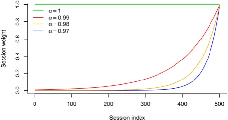
Fig. 1 Session weights at 500th update with fading factors
Fading factors with incremental algorithms can be im-plemented by multiplying the similarity matrix by a fac-torα <1 before each update. In user-based algorithms, the similarity matrix contains similarities measured between ev-ery pair of users in the system. In item-based algorithms, similarities are measured between every pair of items. In both cases, the fading factor causes similarities to contin-uously decrease through time unless they are reinforced by recent session data. If the similarity reaches a lower thresh-old value, it can be assumed to be zero. This method is sim-ple to imsim-plement and requires a single scan of each session. Figure1 illustrates the session weight curve that is ob-tained at session index 500 using different factors. We can observe that the decay for recent sessions is higher than for older sessions. Using forgetting curves with different shapes requires a more complex approach. Because session history is not kept, there is no way to know how to apply forget-ting to each similarity value. Keeping ordered session data in memory would allow us to use different decay curves, however, it would also introduce complexity in the update process. Each session would have to be processed at every update until its weight is zero.
Fading factors can also be implemented in nonincremen-tal algorithms if all considered sessions are kept in memory in the same order by which they arrived. A function of the session index can then be applied when rebuilding the simi-larity matrix, giving less weight to older sessions. However, this poses the same problem of using sliding windows: each session is processed several times, which is undesirable.
4 Algorithms
All algorithms take binary usage data as input. This data contains the set of items visited by each user, grouped in ses-sions and ordered by the session end time. A session is con-sidered to be the set of items visited or rated by a single user in a certain time frame. For the purpose of this work, datasets contain only anonymous users, so each session corresponds to a unique user. Sessions containing a single item are re-moved. Datasets are processed to build a similarity matrix
Sthat contains the similarities between all pairs of users— in the user-based version—or items—in the item-based ver-sion. Similarity between a pair of users (or items) is calcu-lated using a simplified version of the cosine measure for binary ratings [14,15]. IfUandV are the sets of items that usersuandv evaluated, then the user-based similarity be-tweenuandvis given by
sim(u, v)=√#(U∩V )
#U×√#V (1)
For the item-based version, ifIandJare the sets of users that evaluated itemsiorj, the similarity betweeniandj is given by
sim(i, j )=√#(I∩J )
#I×√#J (2)
4.1 Sliding windows
The sliding window approach basically considers the n most recent sessions to build the similarity matrix S. To illustrate, consider a sequence of the first n user sessions {s1, s2, . . . , sn}, each containing a set of items rated by one user. First, S is built from data in sessions {s1, . . . , sn}. Then, for each new sessionsa, the model is rebuilt with data from sessions{sa−n, . . . , sa}, creating a window that slides through data as it arrives.
Algorithm 1 (UBSW) is a classical user-based non-incremental algorithm adapted for using sliding windows. This algorithm takes in a sequence of user sessions L= {s1, s2, . . .}. The firstnsessions are used to build an initial
user vs. user similarity matrixS. Then, for each new user session inL,Sis recalculated using a new window consist-ing of the latestnsessions. Item activation weights are then calculated and theNrecsitems with the highest weights are recommended.
IBSW (Algorithm2) is an item-based version of the non-incremental algorithm, also using sliding windows. This al-gorithm is based on the item-based nonincremental
algo-Algorithm 1UBSW Input:L,Nrecs,n
Output: recommendation list
– InitializeSwith windowW in= {s1, . . . , sn}
– For each new sessionsa∈L,a > n(by userua) – SetW in= {sa−n, . . . , sa}
– (Re)calculateSusing windowW in
– Determine the activation weightWiof each iteminever seen before byua:
Wi=
users in neighborhood of uathat evaluatediS[ua, .]
users in neighborhood ofua
(3)
Algorithm 2IBSW Input:L,Nrecs,n
Output: recommendation list
– InitializeSusing windowW in= {s1, . . . , sn}
– For each new sessionsa∈L,a > n(by userua) – SetW in= {sa−n, . . . , sa}
– (Re)calculateSusing windowW in
– Determine the activation weightWi of each iteminever seen before byua:
Wi=
items in neighborhood evaluated by uaS[i, .]
items in neighborhoodS[i, .]
(4)
– Recommend the N rec items with the highest activation weight
rithm in [15]. As with UBSW, the algorithm takes in a se-quence of user sessionsLand, for each new session, recal-culates an item vs. item similarity matrixSusing a window with the latestnsessions. Then the item weights are calcu-lated and recommendations are provided accordingly. 4.2 Fading factors
Whereas with sliding windows old data is abruptly forgot-ten, the idea of fading factors is to slowly decrease the im-portance of sessions as they grow old. This can be achieved by manipulating the similarity matrixS. Incremental algo-rithms using fading factors simply multiply S by a factor α≤1 before updating them with the active session data. Withα <1, at each new session, older sessions become less important. Withα=1, older data weight is maintained. To incrementally updateSwe also maintain a frequency matrix F with the number of items corated by each pair of users (user-based) or the number of users that corated each pair of items (item-based). The principal diagonal inF gives us the number of items evaluated by each user—in the user-based case—and the number of users that evaluated each item— in the item-based case. The matrixF contains all necessary data to calculate any similarity inS. The values inF are in-cremented by 1 for every pair of items that are contained in the same session (item-based), or for every pair of users that have seen the same item (user-based). Then only the similar-ities inSthat are affected by changes inF are recalculated. Forgetting is obtained by multiplying matrices SandF by a fading factor α <1. When using α=1 no forgetting occurs. It is important thatbothmatricesSandF are multi-plied byα. Because similarities inS are calculated directly from values in F, forgetting must be reflected also in F. Otherwise, every time rows and columns inSwere updated, no forgetting would occur for them. Also, if onlyF is mul-tiplied byα, nonupdated rows and columns inS would not be forgotten.
UBFF (Algorithm3) is a modified version—using fading factors—of the user-based incremental algorithm originally
Algorithm 3UBFF Input:L,Nrecs,α,n Output: recommendation list
– InitializeDwith sessionssi∈Land weights set to 1: D= {s1,1, . . . ,sn,1}
(W Ddenotes the weights inD)
– Initialize matricesSandFusing{s1, . . . , sn} ⊂L
– For each new sessionsa∈L,a > n(by userua) – UpdateD,SandF:
– LetIabe the set of items in sessionsa
– Multiply all values inSandFand past session weights in Dby fading factorα:
S=αS, F=αF, W D=αW D (5)
– AddsatoDwith weight set to 1:Da= sa,1
– Ifuais a new user, add a row and a column toFand toS – Update the row/column ofF corresponding to ua, using
the newD:
Fua,ux=Fua,ux+
#(Ia∩Ix)×W Dx
(6)
– Update the row/column ofScorresponding to userua:
Sua,.=
Fua,.
Fua,ua×
F.,.
(7)
– Determine the activation weightWiof each iteminever seen before byua(Eq. (3))
– Recommend theNrecitems with the highest activation weight toua
described in [15]. A cache matrixF maintains the number of items covisited by every pair of users. Additionally, the databaseDof user sessions and session weights needs to be maintained. This database is required in the matrices update step in order to reflect the forgetting of user sessions and in the recommendation step to retrieve recommendable items from the nearest neighbors. Each elements, w inDis a pair containing session datas and session weight w. The initial weight of each new session is set to 1. Session weights are then multiplied by the fading factorαevery time a new session is processed. This way, sessions loose weight as they grow older.
Values inF are calculated as the number of items simul-taneously present in the active session and every other (past) session. In order to reflect the forgetting of the older ses-sions, this number needs to be multiplied by the weight of the oldest of the two sessions at each cell in the active ses-sion row/column inF. For example, let the first sessions1of
useru1be composed of 2 itemsiandj. Also, let the tenth
sessions10(of useru10) be composed of the same two items
iandj. This would makeFu1,u10=2. However, at session s10, previous session weights are already lower. Specifically,
the weight ofs9isW D9=α, the weight ofs8isW D8=α2,
Algorithm 4IBFF Input:L,Nrecs,α,n Output: recommendation list
– Initialize matricesSandFusing sessions{s1, . . . , sn} ⊂L
– For each new sessionsa∈L,a > n(by userua)
– Determine the activation weightWi of each iteminever seen before byua(Eq. (4))
– Recommend theNrecitems with the highest activation weight toua
– UpdateSandF:
– LetIabe the set of items in sessionsa
– Multiply all values inSandFby a fading factorα
S=αS, F=αF (8)
– For each new item, add a row and column toFand toS – For each pair of items in(i, j )inIa, update the
correspond-ing row/column inF:
Fi,j=Fi,j+1 (9)
– For each itemiainIaupdate the corresponding row (col-umn) ofS:
Sia,.=
Fia,.
Fia,ia×F.,.
(10)
s1 has weightW D1=α9, so this must be reflected in the
cache matrix asFu1,u10=2×α
9.
The incremental item-based algorithm with fading fac-tors (IBFF—Algorithm4) is based on the incremental item-based algorithm in [15]. In order to incrementally updateS we also need save in memory the auxiliary cache matrixF with the number of users that evaluate each pair of items. The principal diagonal gives us the number of users that evaluate each item. Forgetting is obtained the same way as in UBFF, but in this case, the user session database is not required.
One difference between UBFF and IBFF is that with the first, recommendations are performed after updating the model, while with the latter, recommendations are provided before updating the model. With UBFF, the session belong-ing to the active user needs to be processed before the rec-ommendation step because similarities between the active user and other users may not yet be present in S. With IBFF,Salready contains enough information to compute the recommendations before performing the update. UBFF and IBFF are the same algorithms used in previous work [15], with only the changes that are strictly necessary to function with fading factors. This allows us to make comparisons be-tween past and present results.
5 Evaluation and results
In this section, we present results obtained in experiments conducted to evaluate the impact of forgetting mechanisms
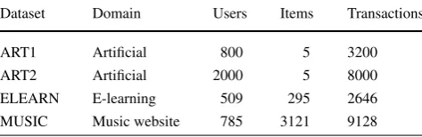
Table 1 Description of the datasets used
Dataset Domain Users Items Transactions
ART1 Artificial 800 5 3200
ART2 Artificial 2000 5 8000
ELEARN E-learning 509 295 2646
MUSIC Music website 785 3121 9128
in CF algorithms. Our main goal is to assess the potential of forgetting mechanisms to improve scalability and predictive ability. We also implement an evaluation methodology that is able to deal with usage data streams. This approach allows us to continuously monitor the behavior of the algorithms.
5.1 Datasets
Four datasets are used in the experiments. Table1describes each dataset. Sessions with less than 2 items were removed. In all datasets, every user performs exactly one session, meaning that each session corresponds to a different unique user.
Datasets ART1 and ART2 are synthesized datasets with an abrupt change. Both ART1 and ART2 consist of identi-cal sessions with 4 items. These sessions contain the items {a, b, c, d}at the beginning and then the itemd is replaced by a new iteme. This change occurs at session index 400 in ART1 and session 500 in ART2.
ELEARN and MUSIC are natural datasets extracted from web usage logs of an e-learning website (ELEARN) and lis-tened tracks from a social network1 dedicated to nonmain-stream music (MUSIC).
5.2 Evaluation methodology
In all experiments we have used theall-but-oneprotocol as described in [3], but following a chronological ordering for sessions. First, the dataset is split in a training set and a test set. Sessions are not selected randomly to the training and test sets, but rather according to their order. This means that for a split of 0.2, for example, the training set is composed of the first 20 % sessions and the test set is composed of the remaining 80 %. For IBSW and UBSW, the training set is considered to be the first window. For IBFF and UBFF, an initial training set containing the first 10 % of sessions is used to build the initial matricesSandF. This initial train-ing set is required in order to avoidcold-startproblems [20]. After splitting the dataset, an item is randomly hidden from each session in the test set. Then recommendations made to each user are evaluated as a hit if the hidden item is among the recommended items.
To evaluate recommendations, we use Precision and Re-call, with the following definition:
Precision= # hits
# recommended items (11)
Recall= # hits
# hidden items (12)
One other possible measure, that combines Precision and Recall, is the F1 measure:
F1=2×Recall×Precision
Recall+Precision (13)
Since one single item from each session is hidden, Recall is either 1 (hit) or 0 (miss), and Precision is obtained divid-ing Recall by the number of recommended items, which is a predefined parameter (see Sect.5.2.1). For this reason, we present predictive ability using Recall only. Precision and/or F1 scores can be easily calculated from Recall and the num-ber of recommended items.
Recall is calculated sequentially for each user. At the end, we obtain a sequence of hits and misses, and an overall av-erage can be calculated. However, as this avav-erage may hide different behaviors through time, we study the evolution of Recall values through time for each experiment. A moving average of Recall is used to obtain values and graphics that illustrate how accuracy varies with time, as new sessions ar-rive. It is important to use this approach because we want to study how Recall evolves with and without implementing forgetting mechanisms. In the Recall graphics, a moving av-erage consisting of the arithmetic mean of the previous 40 Recall values (0 or 1) is used to draw the graphics. In prac-tice, this represents the proportion of hits in the previous 40 recommendation requests.
Computational time spent building or updating the matri-ces is provided for natural datasets ELEARN and MUSIC. Time measurements allow us to empirically study the scala-bility of algorithms using different datasets and parameters. Reaction to sudden changes in data, using natural datasets ELEARN and MUSIC, is studied introducing artificial changes in these datasets. For the purpose of our experi-ments, we randomly chose 50 % of the existing items and change their names from a certain session onwards, causing a suddendrift. The algorithms are then evaluated using these modified datasets. These new datasets keep all the charac-teristics of a natural dataset, only with a drift of 50 % of the items.
5.2.1 Evaluation parameters
The following parameters must be set to conduct the tests: – k: the maximum number of neighbors (users or items) to
consider inSwhen computing recommendations;
– Nrec: the number of items to recommend at each recom-mendation request;
– wp: the window size in percentage of total sessions in the dataset (for IBSW and UBSW);
– α: the fading factor. In IBFF and UBFF,SandF are mul-tiplied by this factor before updating with new data. In the experiments with synthesized datasets (ART1 and ART2), values k=2 and Nrec=1 are used. These low values are chosen because synthesized datasets have a low number (4) of items. With all other datasets values k=5 andN rec=5 are used. These values are chosen taking into account results obtained in [13] and the computational re-sources required to run the experiments.
For the incremental algorithms, four values of α are tested. Values close to 1 are chosen so that the forgetting is not too abrupt. The nonforgetting factorα=1 is used as reference to measure and compare the impact of forgetting with different factors.
To study the impact of forgetting, we compare UBSW and IBSW, which use sliding windows, with their non-forgetting versions that use growing windows. These are called UBGW and IBGW. With growing windows, at each sessionsi, all past sessions{s1, . . . , si−1}are used to buildS.
For UBGW and IBGW, wp is the percentage of sessions used to build the initial matrixS.
Implementation and hardware details All algorithms were implemented using R version 2.11.0 with the packagespam version 0.21–0 to handle sparse matrices. The hardware used in the experiments was a machine with a dual 2.67 GHz core processor and 2Gb of RAM, running the Ubuntu 8.04 Linux OS.
5.3 Experiments with synthesized datasets
Fig. 2 Predictive ability of IBSW and IBFF with ART2. A moving average (n=40) is used to smoothen thelines. For IBSW,wprepresents the percentage of sessions used as learning data. Thevertical dashed lineindicates the point where change occurs
5.4 Experiments with quasinatural datasets 5.4.1 Nonincremental with sliding windows
Figure 3 illustrates the recall levels obtained with UBSW and UBGW. UBSW responds better than UBGW immedi-ately after the change with the ELEARN dataset. With the MUSIC dataset, UBGW almost always outperforms UBSW, although differences between results by both algorithms are small.
With IBSW and IBGW, shown in Fig.4, the experiments with the ELEARN dataset show a better recovery from change with IBSW. This only happens right after change oc-curs. Then, shortly after session 200, IBGW recovers and remains better than IBSW. At the end of the experiment, IBSW drops rapidly to values close to 0.4, while IBGW holds on to values around 0.7.
5.4.2 Incremental with fading factors
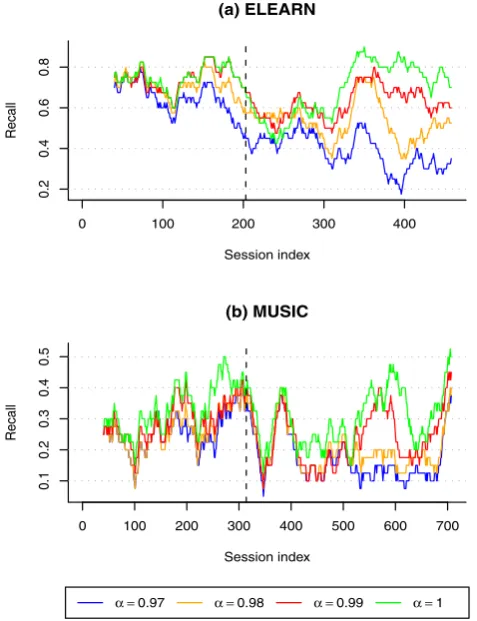
Figure5 shows the reaction of UBFF to change. With the ELEARN dataset, there is a better reaction of the algorithm with lower fading factor. The best results are obtained with α=0.97, from session 200 to around session 450. The second best results are achieved with α=0.98. Analyz-ing the lines in Fig.5(a), from session 200—where change is introduced—to around session 350, Recall is generally higher for lower fading factors. In that interval, the lower recall values are obtained withα=1 (without forgetting).
With the MUSIC dataset (Fig.5(b)) results are very sim-ilar for all 4 fading factors. UBFF withα=1 seems to have a slightly better performance most of the time.
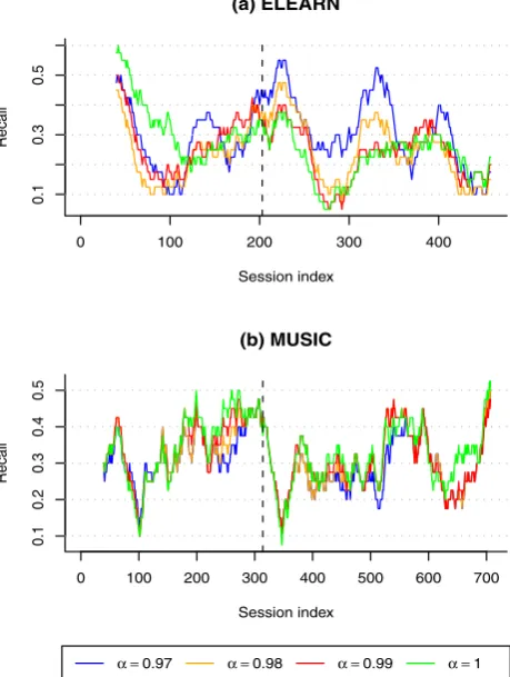
With the item-based version (IBFF), shown in Fig. 6, recall is generally lower with α <1 than withα=1, al-though it is possible to see a better response to change with the ELEARN dataset withα=0.98 andα=0.99 between sessions 200 and 350. With the MUSIC dataset, the highest recall is obtained without forgetting (α=1).
Fig. 3 Comparison between recall of UBSW and UBGW with
w=0.2 and 50 % drift. A moving average (n=40) is used to smoothen the lines. Thevertical dashed linemarks the point where changes are introduced
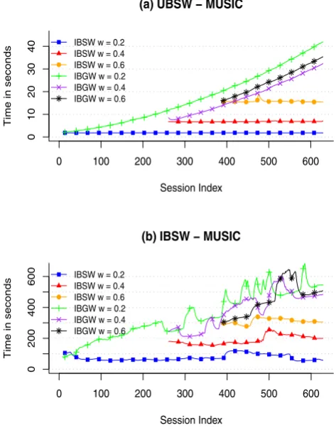
5.5 Update time
Fig. 4 Comparison between recall of IBSW and IBGW withwp=0.2
and 50 % drift. A moving average(n=40)is used to smoothen the lines. Thevertical dashed linemarks the point where changes are in-troduced
case. In the case of matrix rebuild time—for IBSW and UBSW—the similarity matrixSis rebuilt from scratch every time a new session is available. With IBFF and UBFF val-ues in matricesSandF are selectively updated. In any case, these matrices are typically very large and tend to grow very fast as new users and items enter the system. In this section, we study the scalability of the algorithms by measuring the time needed to rebuild or update the similarity matrix. 5.5.1 Nonincremental with sliding windows
Nonincremental algorithms need to recalculate the whole similarity matrix S every time a new session occurs. Fig-ure 7 illustrates the time required to rebuild the matrix as the ELEARN dataset is processed. Comparing the sliding window algorithms with their growing window versions, it is clear that both user-based and item-based versions us-ing growus-ing windows (UBGW and IBGW) time to recal-culateS grows super-linearly with the number of sessions. The sliding window versions tend to maintain time. Com-paring the user-based algorithms with the item-based ones, the first have a more stable record than the latter. This hap-pens because with user-based algorithms,S has exactly the
Fig. 5 Recall of UBFF with 50 % drift. A moving average(n=40)
is used to smoothen thelines. Thevertical dashed linemarks the point where changes are introduced
same number of rows and columns as the number of sessions in the window. With item-based algorithms, the number of items in the window is not fixed—with sliding window—nor it grows one by one—with growing windows—since the or-der of appearance of new items is not sequential. This leads to memory allocation and garbage collection processes to run frequently, causing extra time consumption in some it-erations.
Fig. 6 Recall of IBFF with 50 % drift. A moving average(n=40)is used to smoothen thelines. Thevertical dashed linemarks the point where changes are introduced
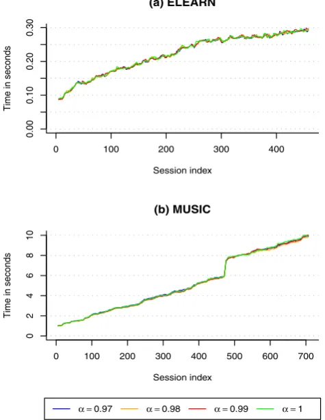
5.5.2 Incremental with fading factors
Incremental CF algorithms, instead of rebuilding the entire similarity matrix, only update the similarity values that can potentially change with a specific session. As shown in [15], this has a considerably lower complexity than a complete rebuild. By looking at the time scales in Figs. 9 (UBFF) and 10—IBFF, and comparing them with those of nonin-cremental algorithms (Figs.7and8), we can verify that in-cremental algorithms—UBFF and IBFF—update times are much shorter than rebuild times by UBSW/UBGW and IBSW/IBGW.
Analyzing UBFF update times in Fig.9, it is clear that time increases as more data is available. Additionally, there seem to be very little differences between runs with different fading factors, includingα=1 (no forgetting). With IBFF (Fig.10), results are also very similar between different fad-ing factors.
Looking at the combination between user-based/item-based and the ELEARN/MUSIC datasets, we observe that with the ELEARN dataset, IBFF performs better than UBFF, while with the MUSIC dataset the opposite occurs. This is an effect similar to the one observed with nonincremental
al-Fig. 7 Matrix rebuild time with nonincremental algorithms (ELEARN dataset). A moving average(n=40)is used to smoothen thelines
gorithms, and again is caused by the proportion of the num-ber of items and users in the datasets.
5.6 Update times with Netflix data
When using fading factors, the matrices S andF become sparser as similarities and cooccurrence frequencies are for-gotten. The algorithms actually take advantage of this spar-sity to optimize the data structures whereSandFare stored, leading to a better scalability. This is not visible in ELEARN and MUSIC because these datasets are not large enough to completely forget similarities and frequencies. However, us-ing a longer dataset it is possible to observe that fadus-ing fac-tors improve scalability. To verify this, we calculate update times of IBFF with a dataset consisting of 5,000 sessions sampled the well-known Netflix Prize [2] dataset.
Fig. 8 Matrix rebuild time with nonincremental algorithms (MUSIC dataset). A moving average(n=40)is used to smoothen thelines
Figure11depicts the update times of IBFF with this sam-ple. It is possible to observe that withα=1 time grows ap-proximately linearly with the number of analysed sessions. Withα <1, the time spent updatingS andF shows a sim-ilar behavior until around session 1600, and then it starts to deviate downward from the nonforgetting configuration. Furthermore, there seems to be a relation between values of α and time gains—lower values require less time. The downsize of this experiment was the overall poor accuracy of the algorithm, with an average recall of 0.021 withα=1 and 0.01 with α=0.99. We believe this is caused by the removal of information (ratings<4) and low representative-ness of the sample.
5.7 Discussion 5.7.1 Predictive ability
Using the ELEARN dataset, forgetting mechanisms provide clear improvements in recall immediately after a sudden drift, except with IBFF, where slight improvements are only obtained with high fading factors (slow forgetting). How-ever, the same is not observable in any case with the MUSIC dataset. With this dataset, immediately after the occurrence of a drift, improvements are not observed, but relative degra-dation is also not present. This contradicts results obtained
Fig. 9 Matrix update time with UBFF. A moving average(n=40)is used to smoothen thelines
with synthesized datasets that suggest a better capability to adapt to sudden drifts. A number of factors can influence the behavior of the algorithms, namely the presence of nat-ural drifts and the natnat-ural variability of the datasets. This motivates further research to understand how dataset inher-ent features such as natural variability and the occurrence of sudden and gradual drifts relate to forgetting parameters such as window length and fading factor values.
5.7.2 Update time
With nonincremental algorithms (UBSW/UBGW and IBSW/IBGW), the first observation is that the sliding win-dow algorithms tend to maintain an approximately constant time to rebuild the matrix, while with growing window al-gorithms time increases throughout the experiment. This is a natural consequence of the use of fixed length windows. The number of sessions to process, in the case of UBSW and IBSW, is fixed, which leads to approximately constant time. Gains in scalability are the most evident motivation for the use of sliding windows.
Fig. 10 Matrix update time with IBFF. A moving average(n=40)is used to smoothen thelines
Fig. 11 Matrix update time with IBFF and data sampled from Netflix. A moving average(n=40)is used to smoothen thelines
means that every window has the same number of users. However, the number of items can vary considerably within each new window. As a consequence, the item-based algo-rithms are more prone to fluctuations in the time required to rebuildS.
Time with the use of fading factors in incremental al-gorithms seems to be unaffected with ELEARN and MU-SIC, but using a longer dataset, it becomes more evident
that fading factors also have the potential to improve scal-ability. With fading factors, older similarity values tend to zero, but it takes a large amount of sessions for similari-ties to actually become zero. The packagespamoptimizes sparse matrix storage by storing only values greater than 2.220446×10⁻¹⁶[7]. For example, withα=0.97, a simi-larity value of 0.5, if never updated by recent data, only gets completely “forgotten” (i.e., becomes zero) after 1,170 ses-sions, which is more than the number of sessions in both ELEARN and MUSIC.
User-based algorithms produce smaller matrices when the number of users is lower than the number of items and larger matrices when the number of users exceeds the num-ber of items. Time to rebuild and/or update these matrices is directly affected by the amount of data to process. This explains why user-based algorithms perform better with the MUSIC dataset, while item-based algorithms have better re-sults with ELEARN.
6 Conclusions
We have implemented and evaluated the impact of forget-ting mechanisms in nonincremental and incremental collab-orative filtering algorithms. Our results suggest that non-incremental algorithms that use sliding windows, when compared to their nonforgetting versions using a grow-ing window, reduce computational requirements while not negatively affecting—and in some situations improving— predictive ability. Results also suggest that incremental al-gorithms benefit from the use of fading factors, although the fading factor approach has more subtle improvements in time requirements. It is also confirmed that incremen-tal algorithms are more scalable than non-incremenincremen-tal algo-rithms.
This work studies the impact of forgetting mechanisms in an abrupt change scenario. Our experimental results were limited with respect to gradual drifts, either due to the data sets we have used or due to limitations of our approach. In the future, we intend to further evaluate forgetting mecha-nisms under both abrupt and gradual drifts. This will require researching how forgetting mechanisms relate to dataset in-trinsic characteristics. A better understanding of datasets will allow the implementation of algorithms that are able to automatically adjust forgetting parameters to different situ-ations. This will allow the implementation of dynamic for-getting, only when useful. We are also working on the im-plementation of the algorithms to allow larger scale exper-iments and the use of fading factors more sporadically— everyksessions.
PONORTE and by the ERDF—European Regional Development Fund through the COMPETE Programme (operational programme for com-petitiveness) and by National Funds through the FCT—Fundação para a Ciência e a Tecnologia (Portuguese Foundation for Science and Tech-nology) within project «FCOMP-01-0124-FEDER-022701».
References
1. Babcock B, Datar M, Motwani R (2002) Sampling from a moving window over streaming data. In: SODA ’02: proceedings of the thirteenth annual ACM-SIAM symposium on discrete algorithms, 6–8 January, 2002, San Francisco, CA, USA. ACM/SIAM, New York, pp 633–634
2. Bennet J, Lanning S (2007) The neflix prize. In: KDD cup and workshop.www.netflixprize.com
3. Breese JS, Heckerman D, Kadie CM (1998) Empirical analysis of predictive algorithms for collaborative filtering. In: Cooper GF, Moral S (eds) UAI ’98: proceedings of the fourteenth conference on uncertainty in artificial intelligence, 24–26 July, 1998, Univer-sity of Wisconsin Business School, Madison, Wisconsin, USA. Morgan Kaufmann, San Mateo, pp 43–52
4. Ding Y, Li X (2005) Time weight collaborative filtering. In: Her-zog O, Schek HJ, Fuhr N, Chowdhury A, Teiken W (eds) CIKM. ACM, New York, pp 485–492
5. Ding Y, Li X, Orlowska ME (2006) Recency-based collaborative filtering. In: Dobbie G, Bailey J (eds) ADC. CRPIT, vol 49. Aus-tralian Comput Soc, pp 99–107
6. Domingos P, Hulten G (2001) Catching up with the data: research issues in mining data streams. In: DMKD ’01: workshop on re-search issues in data mining and knowledge discovery
7. Furrer R, Sain SR (2010) spam: A sparse matrix R package with emphasis on mcmc methods for Gaussian Markov random fields. J Stat Softw 36(10):1–25.http://www.jstatsoft.org/v36/i10/ 8. Gama J, Sebastião R, Rodrigues PP (2009) Issues in evaluation of
stream learning algorithms. In: JFE IV, Fogelman-Soulié F, Flach PA, Zaki MJ (eds) Proceedings of the 15th ACM SIGKDD in-ternational conference on knowledge discovery and data mining, Paris, France, June 28–July 1, 2009. ACM, New York, pp 329– 338
9. Hill WC, Stead L, Rosenstein M, Furnas GW (1995) Recommend-ing and evaluatRecommend-ing choices in a virtual community of use. In: CHI 95 conference proceedings, Denver, Colorado, 7–11 May, 1995, pp 194–201
10. Koren Y (2009) Collaborative filtering with temporal dynamics. In: IV JFE, Fogelman-Soulié F, Flach PA, Zaki MJ (eds) KDD. ACM, New York, pp 447–456
11. Koychev I (2000) Gradual forgetting for adaptation to concept drift. In: Proceedings of ECAI 2000 workshop current issues in spatio-temporal reasoning, pp 101–106
12. Linden G, Smith B, York J (2003) Amazon.com recommenda-tions: item-to-item collaborative filtering. IEEE Internet Comput 7(1):76–80
13. Miranda C (2008) Filtragem colaborativa incremental para re-comendações automáticas na web. Master’s thesis, Faculdade de Economia da Universidade do Porto
14. Miranda C, Jorge AM (2008) Incremental collaborative filtering for binary ratings. In: Web intelligence. IEEE Press, New York, pp 389–392
15. Miranda C, Jorge AM (2009) Item-based and user-based incre-mental collaborative filtering for web recommendations. In: Lopes LS, Lau N, Mariano P, Rocha LM (eds) Proceedings, progress in artificial intelligence, 14th Portuguese conference on artificial in-telligence, EPIA 2009, Aveiro, Portugal, 12–15 October, 2009. Lecture notes in computer science, vol 5816. Springer, Berlin, pp 673–684
16. Nasraoui O, Cerwinske J, Rojas C, González FA (2007) Perfor-mance of recommendation systems in dynamic streaming environ-ments. In: Proceedings of the seventh SIAM international confer-ence on data mining, 26–28 April, 2007, Minneapolis, Minnesota, USA. SIAM, Philadelphia
17. Nasraoui O, Uribe CC, Coronel CR, González FA (2003) Tecno-streams: tracking evolving clusters in noisy data streams with a scalable immune system learning model. In: Proceedings of the 3rd IEEE international conference on data mining (ICDM 2003), 19–22 December 2003, Melbourne, Florida, USA. IEEE Comput Soc, Los Alamitos, pp 235–242
18. Papagelis M, Rousidis I, Plexousakis D, Theoharopoulos E (2005) Incremental collaborative filtering for highly-scalable recommen-dation algorithms. In: Hacid MS, Murray NV, Ras ZW, Tsumoto S (eds) Proceedings, foundations of intelligent systems, 15th in-ternational symposium, ISMIS 2005, Saratoga Springs, NY, USA, May 25–28, 2005. Lecture notes in computer science, vol 3488. Springer, Berlin, pp 553–561
19. Resnick P, Iacovou N, Suchak M, Bergstrom P, Riedl J (1994) Grouplens: an open architecture for collaborative filtering of net-news. In: CSCW ’94, proceedings of the conference on computer supported cooperative work, 22–26 October, 1994, Chapel Hill, NC, USA, pp 175–186
20. Schein AI, Popescul A, Ungar LH, Pennock DM (2002) Methods and metrics for cold-start recommendations. In: SIGIR 2002: pro-ceedings of the 25th annual international ACM SIGIR conference on research and development in information retrieval, 11–15 Au-gust, 2002 Tampere, Finland. ACM, New York, pp 253–260 21. Shardanand U, Maes P (1995) Social information filtering:
algo-rithms for automating “word of mouth”. In: CHI 95 conference proceedings, Denver, Colorado, 7–11 May, 1995. ACM/Addison-Wesley, Reading, pp 210–217