Improving MapReduce privacy
by implementing multi‑dimensional
sensitivity‑based anonymization
Mohammed Al‑Zobbi
*, Seyed Shahrestani and Chun Ruan
Introduction
Conventional data uses anonymity techniques to hide personal information that can cause side link attacks. Anonymization methods, based on k-anonymity, have been widely employed for such purposes [1]. These methods fall into two broad categories. The first category constitutes of techniques that generalize data from the bottom of the taxonomy tree towards its top and are referred to as the bottom-up generalization (BUG) [2]. The second one is based on walking through the taxonomy tree from the top towards the bottom, known as the top-down specialization (TDS) [3]. However, tradi-tional anonymization methods lack scalability and cannot, in general, cope with large sizes of data, as their performance degrades. Hence, a need for scaling up of the conven-tional methods is essential. Scaling up the convenconven-tional methods has resulted in several
Abstract
Big data is predominantly associated with data retrieval, storage, and analytics. Data analytics is prone to privacy violations and data disclosures, which can be partly attrib‑ uted to the multi‑user characteristics of big data environments. Adversaries may link data to external resources, try to access confidential data, or deduce private informa‑ tion from the large number of data pieces that they can obtain. Data anonymization can address some of these concerns by providing tools to mask and can help with con‑ cealing the vulnerable data. Currently available anonymization methods, however, are not capable of accommodating the big data scalability, granularity, and performance in efficient manners. In this paper, we introduce a novel framework that implements SQL‑like Hadoop ecosystems, incorporating Pig Latin with the additional splitting of data. The splitting reduces data masking and increases the information gained from the anonymized data. Our solution provides a fine‑grained masking and conceal‑ ment, which is based on access level privileges of the user. We also introduce a simple classification technique that can accurately measure the anonymization extent in any anonymized data. The results of testing this classification technique and the proposed sensitivity‑based anonymization method using different samples will also be discussed. These results show the significant benefits of the proposed approach, particularly regarding reduced information loss associated with the anonymization processes.
Keywords: Anonymization, Big data, Data privacy, Granular access, Hadoop, MapReduce
Open Access
© The Author(s) 2017. This article is distributed under the terms of the Creative Commons Attribution 4.0 International License (http://creativecommons.org/licenses/by/4.0/), which permits unrestricted use, distribution, and reproduction in any medium, provided you give appropriate credit to the original author(s) and the source, provide a link to the Creative Commons license, and indicate if changes were made.
RESEARCH
*Correspondence:
[email protected] School of Computing,
amendments to these fundamental techniques, including parallel BUG [4], hybrid BUG and TDS [5], and two-phase TDS [6].
All k-anonymity methods identify a set of attributes, known as quasi-identifiers (Q-ID). Q-IDs are attributes that contain private information, where adversaries can use to unveil hidden data by linking them to related external elements [7]. Current anonymization algorithms aim to improve data privacy by generalizing the Q-ID attributes through pro-cesses that utilize taxonomy tree, interval, or suppression. Q-ID attributes are replaced by taxonomy tree values or intervals. The best taxonomy or interval values are named as the best cut. In TDS method, the entropy is used to calculate the highest Q-ID score for the best cut. Other methods implement the median calculation to find out the best cut within the numerical Q-ID attributes [8]. However, these methods do not adequately address the scalability issues. Large data size is an obstacle for these techniques, as they need to fit the data into the limited memory that is available. Processing big data may overwhelm the hardware and result in performance inefficiencies even in parallel computing environ-ments. To overcome such inefficiencies, some techniques split the large size of data ran-domly into small chunks of data blocks, so they can fit into the memory for carrying out the required computations [6]. However, this resolution does not provide a real scalabil-ity solution, since it degrades the performance and increases the masking of anonymized data. These points will be further discussed in “MDSBA groups definitions” section.
We introduce a novel anonymization method using BUG in k-anonymity that can address the scalability and efficiency issues. The method utilizes multi-dimensional sensitivity-based anonymization for data (MDSBA). The main aim of our method is to improve the anonymiza-tion process and to increase the usefulness of anonymized data. MDSBA saves computaanonymiza-tion time, by providing pre-calculated k value, pre-defined Q-ID for anonymization, and pre-cal-culated level of anonymization. To reduce heap memory usage, most current anonymization methods may split large data into small size blocks. The randomness associated with split-ting data into blocks can result in reductions of the usefulness of the processed data. Our method merely splits data, and it is not based on random fragmentation of data. Our iterative split process provides a proper input for the parallel distributed domain. We fragment data horizontally in related to the class value, instead of random fragmentation, which increases anonymization loss. This process is an extension of the approaches reported in [8].
MDSBA method protects the direct record link and Obvious Guess attacks. In the direct record link attack, an adversary may use the Q-ID in a table, say, T, to re-iden-tify the personal information, with the help of an external table, ET, which consists of similar Q-ID attributes. K-anonymity prevents such a linkage by ensuring at least some k records are entirely equivalent. In the Obvious Guess attack, an adversary may eas-ily guess the sensitive attribute, without having to identify the record. Protecting from Obvious Guess attack will be further discussed later.
presents the security solutions for the Obvious Guess attacks. In the last section, we pre-sent our experiments with the proposed MDSBA method along with the results and out-comes of our simulation studies are presented.
Enhanced anonymization: motivations and contributions
Many factors have resulted in more demands for big data analytics. There is a definite need for authorization techniques that can facilitate controlling the user’s access to data in granular fine-grained fashions [9]. For instance, organization’s alliance with business partners, contractors and sub-contractors may increase data access demands for ana-lytics. Also, organizational structures impose variant needs for data access levels. The increasing demand for big data analytics and the lack of framework standardization have urged us to contribute to data analytics security in big data, by establishing a framework that can provide a granular access control for data analytics.
Our MDSBA’s aim is the establishment of a framework that can provide a high scal-ability performance and a robust security protection against privacy violation in data analytics. For the sake of performance, the method is implemented by MapReduce operations. MapReduce is a framework for performing data-intensive computations and data analytics in parallel on commodity computers. Hadoop is one of the most promi-nent MapReduce frameworks that gained popularity in big data analytics. A MapReduce process operates to read and write by its file system, known as Hadoop distributed file system (HDFS). In Hadoop framework, two separate processes are performed; mapping and reducing, or MapReduce. The file system splits files into multiple blocks, and each block is assigned to a mapper that reads data, performs some computation, and emits a list of key/value pairs to a reducer process. Reducer, in turn, combines the values belong-ing to each distinct key accordbelong-ing to some function and writes the results to an output file. Parallel and distributed computing is used for large data size, which may exceed 10’s of Terabytes. The default file system’s block size in Apache Hadoop version 3 is 128 MB [10]. Hadoop version 3’s framework, known by YARN, is divided into a master server or NameNode, and slave servers or DataNodes [11, 12].
Introducing multi‑dimensional sensitivity‑based anonymization
MDSBA adopts Q-ID probability for applying masking of taxonomy tree, interval, or suppression. The probability value is derived from the taxonomy tree concept. The tax-onomy tree T is propagated from the parent node w to some leaf nodes ν. So, the prob-ability of propagation from a parent node is P(w)= 1ν. Figure 5 illustrates probabilities
for each parent node in the education tree. The intervals, also, can be presented by prob-ability values. If a number n was presented in an interval of minimum value Vmin, and maximum value Vmax, then the probability of obtaining that number within the inter-val range is P(n)= (V 1
max−Vmin). For example, for the interval of [15–25[, the probabil-ity is (P = 1/10 = 0.1). This probability concept supports the fine-grained access for multiple users. For such cases, data is split into several groups or domains, and for each group, a different anonymization that depends on the user’s access level, is applied. The anonymization process is managed by the value of sensitivity level ψ, which increases or decreases the information gained from the data. User with a higher value of ψ gain more information, and vice versa. The sensitivity level is determined by two major factors: the sensitivity factor ω and the aging factor τ. Consider a dataset, where k represents the k-anonymity value and k represents the ownership level, which is an instant of k-ano-nymity value. A large value of ownership level implies a weak ownership relation, so the weakest ownership relation is when k=k. That is, the integer values of k and k are such that 2≤k≤k. In other words, low values of k correspond to reduced anonymity as a result of higher ownership relations. The sensitivity factor ω is calculated based on its maximum and the minimum values. The maximum value of ω is defined as:
The minimum value of ω is defined as the product of all Q-IDs probabilities, or: (1) ωmax=maxPqid0
, P
qid1 , P
qid2 , P
qid3
(2) ωmin=
4
i=1
P qidi
.
Based on Eqs. 1 and 2, the value of ω can be found linearly between ωmin and ωmax, as shown in Eq. 3:
Equation 3 presents a linear relation between ω and k values. The equation lowers the value of ω when the user’s k value is high, so that the data anonymity is higher. Users with less privileges are given higher k, while the value of k is constant. We also propose that the lowest value of k should be two to avoid unique re-identification. The anonymi-zation is only applied on external organianonymi-zation’s access. External organianonymi-zations are per-mitted to access an anonymized copy of the original data, while accessing the original data is exclusive to the data owners.
Equation 4 collates both terms of ω and τ to compute the sensitivity level ψ. The sen-sitivity level directly manages user’s access privileges. Higher sensen-sitivity levels lead to upper access ranks, where less data masking and concealments are applied. Also, the sensitive nature of an object can be made lower as its related dataset ages. The aging fac-tor τ affects the sensitivity reversely, with considering the negative values of aging facfac-tor. Based on their owners’ decisions, old objects can be deemed to be less sensitive, and increase ψ as they age. In essence, two factors determine the sensitivity level of the data, the sensitivity factor ω, and the aging factor τ, as described Eq. 4.
Equation 4 is used to calculate the sensitivity level ψ, by establishing the sensitivity level of an object for a given user access level. The masking process tends to find any number close or smaller than the sensitivity value. For instance, if ψ = 0.5, then any value between 0 and 0.5 is acceptable. However, the values closer to ψ improve the informa-tion usefulness and the granularity precision. For instance, the age interval of [10–20[ is derived from ψ = 0.1, while the age interval of [10–12[ is derived from ψ = 0.5. We may notice the accuracy difference between both values of ψ, therefore, assigning the closer value to ψ is essential. The aging factor creates a perturbation to the sensitivity value. This factor becomes more significant as the data age becomes older than a particular age that we refer to as its obsolescence value. Equations 3 and 4 show that the lower sensitiv-ity level requires a higher value of k, which corresponds to lower information gain. In other words, the lower sensitivity levels, correspond to higher anonymization and mask-ing levels of information.
The aging factor τ depends on four different parameters, the object obsolescence value Ø, the aging participation percentage ρ, the object age y, and the sensitivity factor ω. The Ø value is defined as the critical age before the object sensitivity starts to degrade. It can be measured in units of hours, days, weeks, months or years, depending on objects obsolescence speed. However, Ø cannot be given a value smaller than 2, so the value of 1 year, for example, can be replaced by 12 months instead. The aging participation per-centage ρ is an approximation perper-centage chosen by data owners. It measures the aging factor participation in data objects. The aging factor τ can remain constant or decrease linearly. It remains unchanged when the age of the object y is less than its obsolescence value, so it remains constant if y < Ø. On the other hand, if the object age is greater than (3) ω=ωmin+
k−k
ωmax−ωmin
k
.
or equal to its obsolescence value, that is y ≥ Ø, then the sensitivity level increases loga-rithmically, which in turn decreases anonymization level. These two cases manage the aging factor τ, as described by Eq. 5.
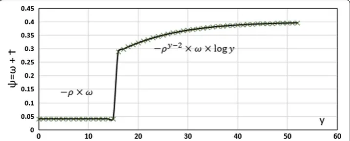
Data owners may set ρ to 0% if their data objects are not affected by time and age. Also, the maximum value of ρ cannot exceed the 90% to avoid a nil value for ψ. It can be noted from Eq. 5 that τ is always negative. In other words, the sensitivity level ψ increases with the age of the information and the passage of time. The newly created data objects result in a lower sensitivity level compared to the old data. In other words, if y < Ø then ψ < ω when the aging factor is incorporated. Equation 5 is derived based on our proposed ideas for incorporating the aging factor and sensitivity analysis for improv-ing the anonymization process. It relies on a linear condition − ρ × ω and a semi-log component (− ρ(y − 2) × ω × logy). The linear part produces a constant value of aging factor when the information has not reached its obsolescence value. The semi-log por-tion is derived from the plotted graph, shown in Fig. 2. The figure illustrates the con-cept that incorporates the age of data objects. Older data is considered to have a logistic degradation with age and passage of time. The degradation starts swiftly before plateau-ing at the sensitivity factor value ω. To illustrate the time factor impact, let us consider the following example: a social media data has an aging participation value set at 0.9 with obsolescence value of 15 days and a sensitivity factor of 0.4 (ρ = 0.9, ω = 0.4, and Ø = 15). Plotting its sensitivity diagram can be initiated by assuming a constant value of sensitivity factor multiplied by the aging participation percentage to find out the aging factor. Therefore, τ = − ρ × ω = − 0.36, and ψ = 0.04. Next, a logistic graph can describe the sensitivity level direct proportions the variable y increase. The sensitivity (5) τ =
−ρ×ω y<∅
−ρ(y−2)×ω×logy y≥ ∅
∅ ∈Z, ∅ ≥0, and y∈Z:y≥2
Fig. 2 Plotted graph to derive Eq. 5 for aging factor: This diagram presents our suggested concept of how the sensitivity value would look like with the aging factor. From this diagram, a mathematical equation was derived as τ=
−ρ×ω y<∅
−ρ(y−2)×ω×logy y≥ ∅ If data owners found that his data importance degrades with
level increases dramatically between days 15 and 30. This sharp increase describes the object degradation importance, which will intentionally reduce the obscurity level on data anonymization.
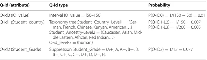
The following example illustrates the calculation steps of sensitivity value ψ. Con-sider an object with three Q-ID attributes, say student IQ test results, similar to those shown in Table 1. The data owner intends to anonymize the data with k = 20, the obso-lescence value Ø is set to 10, the aging participation ρ is 70%, and the age of the object y is13 years. Now, suppose a user was given an ownership value k = 10. Based on the given attributes, the sensitivity level ψ can be calculate using Eqs. 4 and 5. To find out the sensitivity factor ω, it can be noted that the values of ωmax = max (0.01, 0.005, 0.125) is 0.125 and ωmin = 0.01 × 0.005 × 0.125 is 6.25 × 10⁻⁶. The value of ω as per Eq. 3 is ω ≈ 0.063. Based on Eq. 5, the aging factor τ = − (0.7) 11 × 0.063 × log (13) can be seen to be − 0.00138. Therefore, the sensitivity level ψ = 0.063–0.00138 is found to be 0.062.
The previous mathematical equations support the granularity of access control. Our proposed MDSBA is a complete framework that can control both ends of federation service and service providers. Security assertion markup language (SAML) v2 is used to map user’s access level between both ends. The framework consists of three pri-mary services; Core, Initializer, and Anonymizer. The Core service embeds XML files as assertions to transmit the user’s authentication results parallel with the user’s ID, and access level. The access level is determined by delegated roles, while roles are mapped to Q-ID groups. The Initializer service provides initial documents to prepare data for anonymization. The initializer also generates the Pig script line by line, by referring to the provided XML files. Eventually, the Anonymizer service executes the anonymization script remotely. The Initializer operates in the service provider gateway, which is not a member of Hadoop domain. Complete details about the MDSBA framework are further explained in this paper [18].
MDSBA groups definitions
It is evident that records equivalency, in most datasets, increase in parallel with data growth [19]. Therefore, splitting data nominally may increase the data equivalency. Random data split ignores the distribution of equivalent records amongst tables. For instance, in Adult data, patient’s age, sex, and education attributes may appear similar in the first one thousand records, and then related records may appear again at the end of the table. Hence, the random appearance of similar records may reduce the number of equivalency on splitting data into small random chunks, which increases data masking.
Table 1 Three Q‑ID attributes example
Q-id (attribute) Q-id type Probability
Q‑id0 (IQ_value) Interval IQ_value = [50–150] P(Q‑ID0) = 1/(150 − 50) = 0.01 Q‑id1 (Student_country) Taxonomy tree Student_Country_Level1 = {Ger‑
man, French, Chinese, Kenyan, American…} Student_Ancestry‑Level2 = {Caucasian, Asian, Mid‑
dle Eastern, African, Red Indian…} Q‑id_level‑3 = {human}
P(Q‑ID1‑L2) = 1/150 = 0.007 P(Q‑ID1‑L3) = 1/200 = 0.005
Q‑id2 (Student_Grade) Suppression Student_Grade = {A+, A, A−, B+, B,
The following three definitions describe the horizontal split of data by implementing the grouping method of equivalency in MDSBA. We believe that splitting data nomi-nally will increase the equivalency ratio. Suppose a dataset D, with a total number of m attributes, and n records. The data owner defines the number of quasi-identifiers as Q in m attributes, so Q ≤ m. Let some q attributes have equivalent records k, where q attrib-utes are part of Q, so q ≤ Q ≤ m. Hence, the wholly or partly similar records are defined as follows:
Definition 1 All D records are split based on the class C values. Each set of records that contains similar class value is aggregated in a Gi group, where i denotes the number of values appear in the class C. Every Gi group is further processed individually.
Definition 2 The fully-equivalent group (SG) contains some k equivalent records, in some Q attributes. For this group, there is no any anonymization process applied.
Definition 3 The Semi-equivalent group (SSG) contains some k equivalent records, in some q attributes, where 2 ≤ q ≤ Q − 1. The highest Q-IDs probability is usually chosen for q attributes equivalency. The anonymization is applied on the rest of non-equivalent Q-IDs.
Definition 4 The non-equivalent group (NG) contains a number k of equivalent records, in some q attributes, where the number of q = 1. The highest Q-ID probability is usually chosen for q attribute. The anonymization is applied to the rest of non-equiv-alent Q-IDs.
As explained in Definitions 3 and 4, the SSG and NG anonymization is applied on the lowest Q-ID probabilities. For instance, in Adult data the Q-IDs probabilities are; P[Age] = 0.01, P[Sex] = 0.5, P[Edu] = 0.08. Based on these values, the SSG anonymi-zation will be applied on the Q-ID with the lowest probability, which is [Age]. So the semi-equivalency is measured by grouping Sex, and Edu attributes, while Age attribute is anonymized as per interval. The NG anonymization will be applied to all Q-IDs except the one with the highest probability. In our example, the anonymization will be applied to [Edu] and [Age], while records are grouped as per [Sex] equivalency.
directory waiting for stage three. The process starts by reading SSG groups and abstract-ing the non-equivalent groups, denoted by NG. Both of NG and SSG are anonymized by using user defined function Java program.
In Adult data example, Q-ID attributes are grouped by the three Q-IDs (Age, Sex, and Edu), so the number of equivalent records must be greater than or equal to k. These equivalent records are stored in SG, while the equivalent records with a number smaller than k are stored in SSG. In the second stage, the three attributes are grouped again by the largest probability values (Sex, and Edu). The equivalent records with a number greater than or equal to k will be anonymized by Java program. The anonymization is applied on the attribute with the lowest probability value, which is Age. The equivalent records with a number smaller than k are stored in NG, in order to be further grouped and anonymized.
MDSBA and quasi‑identifiers groups
MDSBA presumes a table model with a set of Q-IDs and one sensitive attribute (S), known by a Class. For instance, a table of attributes = {AGE, RACE, STATE, ADDRESS, DISEASE} can be divided into Q-ID = {AGE, RACE, STATE}, and one class of the sensi-tive information S = {DISEASE}.
Definition 5 A table T contains a Q number of Q-IDs, denoted by Q(Q-ID), and a C number of classes, denoted by C(S). Attributes are grouped vertically by dividing Q and C attributes into groups. Each group contains one class attribute and some two to four Q-ID attributes. In other words, 2 ≤ Q(Q-ID) ≤ 4, and C(S) = 1.
MDSBA aims to split data nominally to reduce the data size for the anonymization process by vertically bundling some Q-IDs and Classes into small groups. Many datasets may contain more than one class attribute and a considerable number of Q-IDs. The increased number of Q-IDs may produce a massive computation cost and data overflow, which may unexpectedly terminate the program. Also, bundling small groups of Q-IDs assists the management of access control and authorization. Hence, this technique sup-ports the anonymization performance and scalability. The Q-ID groups are determined by data owners and can be divided randomly or logically. For instance, Seer Cancer Data contains the following attributes = {Sex, Year of Diagnosis, County, State, Grade, Diag-nostic Confirmation, Race, Age}. If the data owner decides to divides attributes to Q-IDs and Classes, then he/she may assign six Q-ID attributes and two categories. Thereby, having two bundles of Q-IDs and one class for each bundle can be a combination of three by three or four by two of Q-IDs. As an example of bundle 1 = {Sex, Race, Age}, and bundle 2 = {year of diagnosis, County, State}, while the classes are; {Grade, Diagnos-tic Confirmation} one per each bundle.
Comparing MDSBA with other anonymization methods
contain data temporarily during the processing tasks and iterations. Programming lan-guages use a limited temporary memory (RAM) during operations, while SQL-like oper-ations are conducted between temporary memory and large repository storage (disk). The SQL-like structure is essential in big data. Implementing programming languages causes high processing costs and low scalable operations. SQL-like also facilitates the handling of large data sizes and leverages the scalability during the analytics process. Anonymization is an example of high-cost operations that needs SQL-like to relieve data overflow over the memory limitations [21].
MapReduce ecosystems, such as Pig and Hive, implement SQL-like as a prominent solution for data flow platform. Apache Pig provides nested data types like tuples, bags, and maps that are not available in MapReduce. Pig provides many built-in operators to support data operations like joins, filters, orders, sort, and others. Whereas performing the same function in MapReduce is a complicated task. Pig compiler manages the data flow by creating a group of tuples or bags. The data group is emitted to YARN container for further processing. If the data group exceeded the memory size, then it spills the retained data to the disk. This kind of management cannot be applied efficiently on the current anonymization methods, such as MDTDS. The reason for that is the limitations of Hadoop ecosystems on dealing with large data flow with multiple conditional itera-tions. Pig, for instance, implements UDF to overcome the Pig programming limitaitera-tions. However, the UDF functions operate in external JVMs, which are not related to YARN platform. UDF transmits data to a black-box that is not able to apply parallelism and a proper data management. Usually, the local JVM may fail to utilize the large size of data in memory, as a reason of the limited Java Heap memory. Therefore, developers should tackle this concern by reducing the UDF use, and minimize the data size processed by UDF [22].
Figure 3 compares between MDSBA and TDS algorithms. The comparison shows the absolute dependence of TDS algorithm on UDF. In TDS, the conditional iteration is nec-essary to find out the best Q-ID score to be specialized. Also, the level of specialization is unknown, so a continuous iteration is needed before finding the best cut. On the con-trary, MDSBA pre-determines the Q-IDs that needed to be anonymized, and the level of anonymization. This saves iteration and computation times. Moreover, MDSBA reduces the data size processed by UDF. This is essential to avoid Java Heap memory error, which may unexpectedly terminate the anonymization process.
prospect. This gives data miners a flexibility of approximating and rounding some num-bers to a few decimal places [23]. Therefore, pre-calculating the k value, and pre-deter-mining the attributes needed to be anonymized is an advantage. This non-accuracy will not dramatically affect the data analytics results.
MDSBA implementation example
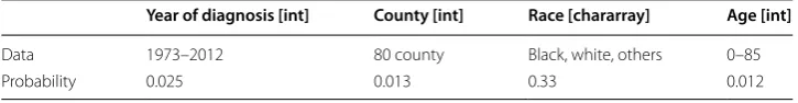
Let us study the following complete example of anonymizing data by implementing Pig Latin script. We will apply anonymization on Seer Cancer Data. Table 2 shows the sug-gested Q-IDs, and the probability for each attribute and Table 3 shows the Class attrib-utes with four sensitive values.
Suppose that data owner assigns k = 400, and aging factor τ = − 0.02. A user attempts to access this data with an ownership level k = 250. Referring to Table 2, and Eqs. 1–3, the ωmax = 0.33, ωmin = 2.5 × 10−06, so the sensitivity factor is found to be ω = 0.124.
Fig. 3 Comparison between the anonymization algorithms of MDSBA and TDS. This figure compares between both anonymization methods, by showing each algorithm’s dependency on UDF. The figure shows a large dependence by TDS, and a low dependence by MDSBA
Table 2 Seer Cancer Data Q‑IDs and probability
Year of diagnosis [int] County [int] Race [chararray] Age [int]
Data 1973–2012 80 county Black, white, others 0–85
The data will be anonymized with a sensitivity level ψ = ω + τ = 0.124 − 0.02 ≈ 0.122. This sensitivity level indicates anonymization degree that will be applied on attributes. For instance, if four numerical Q-ID attributes need to be anonymized, then each attrib-ute can be rewritten by a minimum interval distance of 2. Hence, the factorial result for the four attributes is 1
2×12×12×12 =0.063, which is accepted value since it is smaller than ψ = 0.122. Therefore, if the anonymization was applied on the four numerical Q-IDs, then the year of diagnosis can be given intervals of 2 such as (1973–1975), and similar interval can be applied to the rest of the anonymized attributes. However, the interval distance is determined based on the minimum and maximum numerical value, within the semi-equivalent group. This interval is determined by the UDF program.
Figure 4 is divided into five main stages. Each stage generates a set of groups. Stage Zero aims to flesh out records related to the Obvious Guess. Stage One filters or splits Table 3 Seer Cancer Data class (four sensitive values)
Diagnostic
No positive histology Positive histology
Positive microscopic confirm Positive laboratory test
data based on class values to generate G groups. This is implemented by loading data from HDFS location, before the splitting, so each class value is assigned to one G group. Each G group is then stored separately. After creating G groups, a (group by) command is applied to all Q-ID attributes for each G group. In the four Q-ID attributes case, four Q-ID attributes are grouped for equivalency. The idea is grouping all Q-ID attributes to filter the entirely equivalent records and store them in SG location. The non-equivalent records are stored in a separate SSG1 location. In stage two, three Q-ID attributes of SSG1 data will be grouped for semi-equivalency. The chosen three Q-IDs for grouping have the highest Q-ID probabilities. The records that pass the semi-equivalency criteria are further anonymized. The anonymization is applied on the lowest probability value of Q-ID attribute and finally, stored in SG location. The records that fail the semi-equiv-alency criteria are stored in an SSG2 location for the next stage. In stage three, a simi-lar concept is applied to a semi-equivalent group, before applying anonymization. The grouping command will be implemented for the highest probability values of two Q-ID attributes, while the lowest two probability values are anonymized. However, in all previ-ous stages, the grouping command is cumbersome. The command alters the records for-mat and transposes data from horizontal to vertical. Hence, the grouped records cannot be re-grouped [21]. Therefore, we need a program that can adjust the grouped records back to their original format. A UDF Java program reads the data as bags and converts them back to tuples, named (ADJUST.java). All grouping processes are filtered by com-paring their number of records with the k value, if it is larger, then an anonymization will take a place. Stage two filters three Q-ID attributes of SSG1 data, so if cnt ≥ k, then SSG_P1 Java program will anonymize data before storing it in SG group. Otherwise, data is stored in SSG2 group for the next stage. In stage three, SSG2 data will be grouped by the largest two Q-ID attributes. Data, then, will be anonymized by SSG_P2. In the final fifth stage, records are grouped by the highest QID probability and anonymized either by NG_P if ≥ k, or by SUP_P if < k. A complete Pig script for Adult data is available in Appendix 1, with three Q-ID attributes.
Six UDF Java programs are defined in this process: SSG_P1, SSG_P2, NG_P, SUP_P, OBV_G and ADJUST. The first three programs anonymize data by one Q-ID attribute as in SSG_P1, or by two Q-ID attributes as in SSG_P2, or by three Q-ID attributes as in NG_P. The program SUP_P suppresses all Q-ID attributes as a last resort, where one Q-ID grouping does not meet the k-anonymity criteria. The program SSG_P2 is only
used when the number of Q-ID = 3. The program NG_P may anonymize 1, 2, or 3
attributes, when the total number of Q-IDs is 2, 3, or 4 simultaneously.
Protection from Obvious Guess
MDSBA applies the security protections before executing any grouping operations. The process can be divided into three sub-processes. Initial verification is executed in Pig Latin. The steps include, grouping all Q-IDs, while the class attribute is excluded, and transferring any group number ≥ k to UDF program. The UDF executes the rest of the two sub-processes. These sub-processes are naïve and should not cost extra RAM. The first statement is if statement, to find out if a single class value is found. If yes, then store data in a temp_file over HDFS. If more than one class value is found, then store data in SSG group, so it will ready for Stage two. As described in Fig. 5. Our goal is reducing the number of arrays and iteration processes inside UDF Java program. This is important concept, since Pig Latin was designed to spill out of JVM memory to the disk. However, Java program cannot spill to the disk, so Java heap memory may terminate the program. Hence, we kept the processing cost, with this massive data flow, to the minimal level. Table 4 Obvious Guess example
Year of diagnosis County Race Age Diagnostic
1997 125 Black 25 Positive histology
1997 125 Black 25 Positive histology
1997 125 Black 25 Positive histology
Anonymization classification
Many techniques have been implemented to measure the performance of the anonymi-zation methods. Techniques, usually compare data before and after anonymianonymi-zation to ascertain the information loss. One of the most widely used approaches relevant to information loss is based on measuring the entropy of data after anonymization by cal-culating the tuples fraction in each block of anonymized data, as in Eq. 6.
where T(qi, s) is the tuples fractions in qi blocks and s denotes the sensitive attribute. The entropy then is used with the score equation Score(v)= AnonyLossInfoGain((vv))+1, which defines the relation between information gained and anonymization loss. As shown in Eq. 7, the information gained adopts the entropy equation [24].
The score equation was developed for multi-dimensional top-down specialization (MDTDS), where data blocks are specialized or generalized by implementing Eqs. 6 and 7. Other techniques implement the decision tree by building a cost matrix to find out the classification costs and errors. This technique is usually executed by Naïve Bayes classi-fier or by C 4.5 classiclassi-fiers [25]. However, these techniques predict decisions before and after anonymization instead of finding the actual degradation of data usefulness after anonymization.
We adopted an alternative naïve equation that measures the percentages of infor-mation loss after anonymization, denoted by Disruption (Ɗ). The disruption value is a benchmark that gives a general indication of the size of anonymization loss. As shown in Eqs. 8 and 9, each anonymized block of tuples is calculated individually, and finally, the Ɗ value is the result of the total summation of all anonymized blocks s. Each block of data is a data bag produced by grouping a set of tuples. Let us assume that an anonymized block of data contains some M records, in a total number of N dataset records.
where
P[QID] is the factor of Q-IDs probabilities used in anonymizing each block.
Equation 8 is derived from the reverse proportion between the Q-ID probability and Ɗ. The Ɗ value increases with the increasing number of Q-ID attributes that participate in anonymization. Hence, implementing three anonymized Q-IDs will result in a higher Ɗ value than implementing two anonymized Q-IDs. The following example illustrates (6)
E(T[v])=
s∈S
T[qi,s] log(T[qi,s])
(7)
InfoGain(v)=E(T[v])− c
|T[c]| |T [v]|E(T[c])
(8) Ds= M
N ×
0.01
P[QID]
(9) D[total]=
i
s=0
Eqs. 8 and 9. Recalling the adult data, and considering the total number of records is 500. Two blocks of data were anonymized by two Q-IDs of education and sex. The number of anonymized records for these two blocks was 15 and 30 respectively. The education anonymization was given level 2, which relates to (certificate) and (degree), respec-tively. Based on the EDU taxonomy tree, as shown in Fig. 6; the first block probability is P[EDU] = 0.067 and the second block probability is P[EDU]=0.17. Also, the SEX probability is P[SEX] =0.5. Based on the previous two equations and the given infor-mation, the value of Ɗ is calculated as Ɗ1 = (15 × 0.01)/(500 × 0.067 × 0.5) = 0.009, and Ɗ2 = (30 × 0.01)/(500 × 0.17 × 0.5) = 0.007. Referring to Eq. 9, the total value of Ɗ = 0.016.
Validation and simulation analysis
Our first objective is to evaluate the level of information loss in MDSBA and to compare it with the other anonymization methods. All experiments were performed on our uni-versity Hadoop lab, which includes four virtual machines, with one NameNode and three DataNodes. Each node’s CPU is Intel(R) Xeon(R) CPU E5-2665 0 @ 2.40 GHz × 86_64, with a physical memory of 8 GB. The operating system is CentOS 7 configured with Hadoop version 2, and Pig Latin version 0.15.0. Four different common data were used in our experiments including, adult data, Seer Cancer Data, Heart Disease Data, and Kasandr dataset. Each dataset was randomly enlarged up to three size varieties; these are 1.2, 3.3, and 4.6 GB. The enlargement was created by applying Excel VBA script to produce tens of (.csv) files.
Seer Cancer Data of Q-IDs and the class are described in Tables 2 and 3. Adult
data Q-IDs = {Age, Edu, Sex} and the class is salary = {<= 50 K, > 50 K}. Also, Heart Disease Data Q-ID = {Age, Sex, Smoker, cp}, and the class of electrocardiographic results, i.e., restecg = {normal, having ST-T wave abnormality, and showing probable
or definite left ventricular hypertrophy}. The Kasandr dataset consists of the following attributes = {userid, offerid, city, category, merchant, purchase_date, implicit_feed-back}. For security reasons, the user id is omitted, and the chosen Q-ID = {city, category, purchasedate}. The class is divided based on the 738 types of the merchant. The data-set of Kasandr was collected in Germany. The cities of Germany are around 80 cities, and the products category is around 50 types, while the purchase date was recorded for 5 years over 365 days per annum. Based on these numbers the probabilities are given as; city = 0.0125, category = 0.02, and the date = 0.0005.
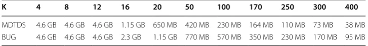
In our experiments, we implemented Java as a UDF combined with Pig scripts. The script reads the database by using Hadoop reading process through HDFS. We divided our three experiments into three sections; MDTDS, BUG, and MDSBA. Both BUG and MDTDS methods were conducted by coding a Java program embedded within Pig script as a registered JAR. However, both methods, BUG, and MDTDS, were executed several times to avoid Hadoop job failure. To prevent this failure, we split the large file gradually into smaller files to overcome the unexpected error occurrences. There was no need to split the large files when the value of k < 16. The number of splits has increased parallel with the increasing value of k. The data split for 4.6 GB dataset is illustrated in Table 4. A separate task processes each small data file. The split is essential to reduce the data over-flow across the UDF program. BUG method performed better with a more significant data size, as shown in Table 5.
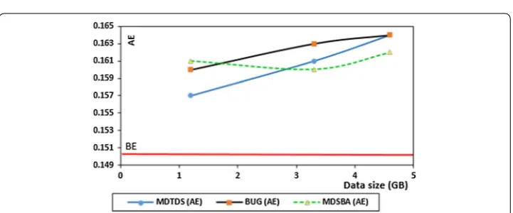
Our first experiment implements a commonly available classifier for comparison between the three anonymization methods. The first comparison relies on Naïve Bayes-ian classifier. We applied anonymization on two datasets, Adult and Seer datasets. After completing the anonymization processes for each dataset, we first calculated the clas-sification error by using RapidMiner Studio. The calculation was conducted before and after the anonymization. We implemented similar testing concept as in [3]. The clas-sification error before anonymity is called Baseline Error and denoted by BE, while after anonymity is called Anonymity Error and denoted by AE. The BE classification error is 0.18 for Adult data, and 0.15 for Seer data. Figures 7 and 8 show the classification error comparison between the three anonymization methods. The comparison considered k = 15 in all trials. Three different data sizes were compared in the three anonymization methods.
Both datasets show similar results regarding AE value. The anonymization was con-ducted based on splitting data in BUG and MDTDS, while data was processed as a whole set in MDSBA. Table 5 illustrates the data split for 4.6 GB. In our trails, the first data size was small enough to avoid data split. Hence, the classification error was low. The low classification error indicates the high level of information gain. However, since data size increases, the anonymization algorithms need to split large data size into small blocks. This split affects the data equivalency to a certain extent. It was also noticed that
Table 5 Dataset of 4.6 GB split for both methods
K 4 8 12 16 20 50 100 170 250 300 400
BUG and MDTDS perform better in smaller data size. This is because of their own algo-rithm’s nature of keeping iteration and splitting until no further split is possible. In both trials, the value of AE showed a slight decline in MDSBA, as a reason of the equivalency increase parallel with the data size increase.
The first experiment does not accurately measure the amount of disruption. The out-put results rely on the classifier accuracy and its efficiency with such a data type. Our second experiment recalled our naïve disruption equation instead of measuring the prediction error percentage. The four datasets are used with 4.6 GB size of each. The anonymization methods are implemented by Bottom-Up Generalization, Top-Down Specialization, and MDSBA. Equations 8 and 9 are used to calculate Ɗ. The first part of the experiment aimed to measure the disruption values for the smaller values of k = 4, while the second part aimed to measure the disruption values for the larger values of
Fig. 7 Disruption comparison for k= 4 and the three data. We developed an equation to find a benchmark for the level of information loss, or the anonymization impact. Named as Disruption. This diagram shows four different datasets; Adult, Seer cancer, Heart disease data and Kasandr. Each dataset was anonymized by Top‑Down specialization, Bottom Up Generalization, and our MDSBA. It was found that our method was the lowest Disrupted
k = 50. Figure 9 shows the results of the first part of the experiment, which indicates a minor contrast between the three methods. MDSBA shows a higher disruption than the others. However, the difference being around 0.0004 is very small and does not have any real impact on data analytics. Figure 10, shows the results of the second part of the experiment, which indicates a significant contrast between the three methods. MDSBA shows the lowest disruption level when k = 50.
In the second experiment, we aimed to find the anonymization level in MDSBA on the variation of k. Figure 11 shows a gradual increase in Ɗ on k ≥ 50 for all dataset. This
Ɗ increase is expected as a reason of the equivalency decrease with the large number of k. This experiment was conducted with a data size of 4.6 GB for each dataset. The k increase may reduce the privacy violation risk, but however, it degrades the informa-tion usefulness. Hence, a tradeoff between security and disrupinforma-tion should be considered on assigning the values of k. From our previous and current experiments, we applied
Fig. 9 The relationship between Ɗ and k variation in MDSBA. Similar to Fig. 6. The Disruption value has increased parallel with the increased value of k
anonymization on verities of datasets, and we found that anonymizing most datasets will output a Ɗ below 5%. However, this finding is a rough estimate and cannot be gen-eralized to all datasets. Data Ɗ is related to other factors, such as the data cumulative distribution, and the attributes probabilities, as described before. Also, low probability attributes are prone to a higher level of anonymization.
In the last experiment, we compared the processing time of MDSBA and MDTDS in Seer Cancer dataset, with the variations of k and data size. The value of k was replaced
with k in MDTDS case, since MDTDS does not implement k. MDTDS data was split
into small size of data files, as shown in Table 5. As illustrated in Fig. 12, MDSBA pro-cessing time is a prominent in small values of k. However, MDTDS has lower latency on larger values of k, while MDSBA consumed the same time in both values of k, when k =50, or k=250. This fixed timestamp refers to the time consumed on applying the Obvious Guess. Larger values of k requires less time spent on Obvious Guess processing, and more time on anonymization processing, and vice versa. Hence, the total of both processing times remains close similar for all k values.
The three experiments showed promising results in performance and security regarding MDSBA. Increasing k value lowered the disruption results. This is essential in big data security, which depends on a higher equivalency number. MDSBA cannot accept smaller values of k, because its core structure relies on the gradual value of k value. This means that the minimum accepted k value cannot be smaller than k = 20. The reason for that is the minimum value of k is 2, and if a user was given 10% of k,
Fig. 11 The relationship between Ɗ and variation in MDSBA
then k = 20 × 0.1 = 2 [18]. However, more experiments are needed to prove MDSBA’s performance and security. Previous experiments were conducted on MDSBA and com-pared with several BUG and MDTDS methods. The experiments showed similar results in information gain results and performance improvement [26].
Conclusions
Big data analytics require proper anonymization tools and methods that furnish for secure procurement of information. Current anonymization methods may not be able to process large data sizes efficiently. Some of the anonymization methods are not capable of discriminating between the roles and potentially different access privilege levels of the users, resulting in the same levels of the information obscurity for their clients. To over-come some of these limitations, in this work, we have proposed a novel sensitivity-based on anonymization framework, MDSBA. The framework provides capabilities for effi-cient anonymization of big data, by incorporating contemporary anonymization tools, such as Pig Latin and UDF programming. Pig Latin shell behaves similar to SQL struc-ture and can speed up the MapReduce operations, by grouping, filtering and splitting of data. Our proposed method can provide an output with various anonymization levels for users with multi-level of access rights. By adopting a bottom-up approach, our anonymi-zation method reduces the rate of the anonymianonymi-zation loss. We have also made simple analytical comparisons of the obscurity levels of data provided by MDSBA, BUG, and TDS. The experiments, with three different datasets, have confirmed that information loss in MDSBA is 1.8 times lower than in MDTDS, and 0.5 times lower than in BUG, with the large values of k. The experiments have also shown the control of the degree of anonymity and data obscurity levels can be easily achieved by managing the MDSBA parameters. MDSBA, also, has shown a low time latency on anonymization process with low values of k. Our future works will expand our experiments to include more sophis-ticated and complex settings to fine-tune the proposed approach. We also aim to estab-lish a complete MDSBA framework, by providing supporting procedures that enhance the fine-grained access control between Federation Services and data Service provid-ers. Moreover, we need to evaluate MDSBA performance in data stream model, since all current studies focus on data batch only. This may require continuous operations to apply anonymity on newly updated data records. Also, our gauge will evaluate MDSBA in various database frameworks, such as Spark and Storm. In addition, further studies are required to find the optimal values of k and k.
Abbreviations
TDS: top‑down specialization; BUG: bottom‑up generalization; Q‑ID: quasi identifier; MDSBA: multi‑dimensional sensitivity‑based anonymization; HDFS: hadoop distributed file system; UDF: user‑defined function; k: ownership level; ω: sensitivity factor; ψ: sensitivity level; Ø: obsolescence value; τ: aging factor; ρ: aging participation percentage; SG: fully‑ equivalent group; SSG: semi‑equivalent group; NG: non‑equivalent group; Ɗ: disruption.
Authors’ contributions
MAZ wrote the main manuscript and the diagrams. CR participated in the set‑up of the experiments and output results. SS reviewed and amended the manuscript scientifically, grammatically, and general text structure. All authors read and approved the final manuscript.
Acknowledgements
Competing interests
The authors declare that they have no competing interests.
Availability of data and materials
Our experiments utilize three different standard datasets. They are: Adults data, taken from UCI machine learning ftp:// ftp.ics.uci.edu/pub/machine‑learning‑databases/adult/adult.data. Seer Cancer Data, data is taken from SEERSTAT soft‑ ware, which is available on https://seer.cancer.gov/seerstat/software/. Kasandr data, taken from UCI machine learning https://archive.ics.uci.edu/ml/datasets/KASANDR. Heart Disease Data, taken from UCI machine learning available at https://archive.ics.uci.edu/ml/datasets/Heart+Disease.
Consent for publication Not applicable.
Ethics approval and consent to participate Not applicable.
Funding
The research works reported in this paper are part of the first author’s Ph.D. degree pursued at Western Sydney Univer‑ sity. The second and third authors are the supervisors of those works. The Australian government partially covers the funding for that degree under the Research Training Scheme (RTS).
Publisher’s Note
Springer Nature remains neutral with regard to jurisdictional claims in published maps and institutional affiliations.
Received: 24 August 2017 Accepted: 17 November 2017
References
1. Sweeney L. Anonymity: a model for protecting privacy. Int J Uncertain Fuzziness Knowl‑Based Syst. 2002;10(05):557– 70. https://doi.org/10.1142/S0218488502001648.
2. Wang K, Yu PS, Chakraborty S. Bottom‑up generalization: a data mining solution to privacy protection. USA; 2004. p. 249–56.
3. Fung BCM, Wang K, Yu PS. Top‑down specialization for information and privacy preservation. USA; 2005. p. 205–16. 4. Irudayasamy A, Arockiam L. Parallel bottom‑up generalization approach for data anonymization using map reduce
for security of data in public cloud. Indian J Sci Technol. 2015;8(22):1.
5. Zhang X, Liu C, Yang C, Chen J, Nepal S, Dou W. A hybrid approach for scalable sub‑tree anonymization over big data using MapReduce on cloud. J Comput Syst. 2014;80:1008–20.
6. Zhang X, Yang LT, Liu C, Chen J. A scalable two‑phase top‑down specialization approach for data anonymization using MapReduce on cloud. IEEE Trans Parallel Distrib Syst. 2014;25(2):363–73.
7. Sun Y, Yin L, Liu L, Xin S. Toward inference attacks for k‑anonymity. Pers Ubiquit Comput. 2014;18(8):1871–80. 8. Zhang X, Yang C, Nepal S, Liu C, Dou W, Chen J. A MapReduce based approach of scalable multidimensional
anonymization for big data privacy preservation on cloud; 2013. p. 105–12.
9. Shtern M, Simmons B, Smit M, Litoiu M. Toward an ecosystem for precision sharing of segmented Big Data. In: Cloud Computing (CLOUD), 2013 IEEE Sixth International Conference on. IEEE; 2013. p. 335–42.
10. Wu X, Zhu X, Wu GQ, Ding W. Data mining with big data. IEEE Trans Knowl Data Eng. 2014;26(1):97–107. 11. Kwon Y. Hadoop internals. Lecture notes from Washington University; 2014. https://courses.cs.washington.edu/
courses/cse344/11sp/lectures/cse344‑guest‑yckwon.pdf. Accessed 10 Feb 2017.
12. Project H. HDFS users guide. Apache. https://hadoop.apache.org/docs/r2.7.2/hadoop‑project‑dist/hadoop‑hdfs/ HdfsUserGuide.html (2016). Accessed 2016.
13. Dokeroglu T, Ozal S, Bayir MA, Cinar MS, Cosar A. Improving the performance of Hadoop Hive by sharing scan and computation tasks. J Cloud Comput. 2014;3(1):1.
14. Gold S. Python: Python programming learn Python programming in a day‑a comprehensive introduction to the basics of Python & computer programming. ACM Digital Library; 2016. https://dl.acm.org/citation.cfm?id=3055663. Accessed 20 Apr 2017.
15. Grimmer M. ‘High‑performance language interoperability in multi‑language runtimes. In: Proceedings of the com‑ panion publication of the 2014 ACM SIGPLAN conference on systems, programming, and applications: software for humanity. ACM; 2014. p. 17–9.
16. Davis AL. Modern programming made easy: using Java, Scala, Groovy, and JavaScript. Berkeley: Apress; 2016. 17. Lublinsky B. Professional hadoop solutions. Hoboken: Wiley; 2013.
18. Al‑Zobbi M, Shahrestani S, Ruan C. Implementing a framework for big data anonymity and analytics access control. In: Trustcom/BigDataSE/ICESS, 2017 IEEE. IEEE; 2017. p. 873–80.
19. Al‑Zobbi M, Shahrestani S, Ruan C. Sensitivity‑based anonymization of big data. In: Local computer networks work‑ shops (LCN workshops), 2016 IEEE 41st Conference on. IEEE; 2016. p. 58–64.
20. Harrington JL. SQL clearly explained. Burlington: Morgan Kaufmann; 2003. 21. Pasupuleti P. Pig design patterns. Birmingham: Packt Publishing; 2014.
22. Li K, Reichenbach C, Smaragdakis Y, Diao Y, Csallner C. SEDGE: symbolic example data generation for dataflow programs. In: Automated software engineering (ASE), 2013 IEEE/ACM 28th International Conference on. IEEE; 2013. p. 235–45.
23. Govindaraju V. Big data analytics. Oxford: Elsevier Science; 2015.
24. Fung BCM, Wang K, Philip SY. Anonymizing classification data for privacy preservation. IEEE Trans Knowl Data Eng. 2007. https://doi.org/10.1109/TKDE.2007.1015.
25. Guller M. Big data analytics with spark a practitioner’s guide to using spark for large scale data analysis. Berkeley: Apress; 2015.