R E S E A R C H P A P E R
Open Access
Sample-based integrated background
subtraction and shadow detection
Arun Varghese
*and Sreelekha G
Abstract
This paper presents an integrated background subtraction and shadow detection algorithm to identify background, shadow, and foreground regions in a video sequence, a fundamental task in video analytics. The background is modeled at pixel level with a collection of previously observed background pixel values. An input pixel is classified as background if it finds the required number of matches with the samples in the model. The number of matches required with the samples in the model to classify an incoming pixel as background is continuously adapted at pixel level according to the stability of pixel observations over time, thereby making better use of samples in dynamic as well as stable regions of the background. Pixels which are not classified as background in the background subtraction step are compared with a pixel-level shadow model. The shadow model is similar to the background model in that it consists of actually observed shadowed pixel values. Sample-based shadow modeling is a novel approach that solves the highly difficult problem of accurately modeling all types of shadows. Shadow detection by matching with the samples in the model exploits the recurrence of similar shadow values at pixel level. Evaluation tests on various public datasets demonstrate near state-of-the-art background subtraction and state-of-the-art shadow detection
performance. Even though the proposed method contains shadow detection processing, the implementation cost is small compared with existing methods.
Keywords: Background subtraction, Change detection, Shadow detection
1 Introduction
The use of change detection algorithms to automati-cally segment a video sequence from a stationary camera into background and foreground regions is a crucial first step in several computer vision applications. Results from this low-level task are often used for higher level tasks such as tracking, counting, recognition, and classification. The foreground regions correspond to the objects of our interest, for example, vehicles or people. In a real-world scenario, there are several problems which make change detection a more challenging problem than a simple moving/static classification. One is dynamic background which are regions in the background exhibiting nuisance motion like tree branches or flags swaying in the wind, ripples on water, and fountains. A good change detec-tion algorithm should classify such regions of irrelevant motion as background to exclude them from further analysis.
*Correspondence: [email protected]
Department of Electronics and Communication Engineering, National Institute of Technology, Calicut, India
Another concern for change detection algorithms is intermittent object motion. A foreground object which temporarily becomes static is to be retained in the fore-ground (e.g., a car stopped at traffic light or a person standing still). A related challenge is that of moved back-ground objects.
An additional major challenge for change detection algorithms is presented by cast shadows which accom-pany foreground objects. Unless explicit handling is done, background subtraction algorithms tend to classify cast shadows as part of the foreground, detrimental to the subsequent stages of analysis. For example, in an intelli-gent traffic surveillance system, shadows can distort the shape of detected vehicles or cause multiple vehicles to be merged into one, which often leads to failure in subse-quent content analysis steps.
The most common method for foreground segmenta-tion isbackground subtraction. Modern background sub-traction algorithms operate by first building a model for the background. An incoming frame is compared with the background model, and every pixel in the frame is clas-sified as either background or foreground based on the
similarity with the model. Pixels in the current frame that have significant disparities with the model are labeled as foreground. An incoming frame is also used to update the background model. Updating the background model is necessary since the model should adapt to various changes in the background like gradual or sudden illumi-nation changes (changing time of the day, toggling of light switch, etc.), weather changes (rain, fog, etc.), or struc-tural changes in the background. Most algorithms employ independent pixel-wise models for the background to aid fast hardware implementations. Post-processing opera-tions like morphological or median filtering are often used to ensure some spatial consistency to the segmentation results.
2 Related methods
2.1 Background subtraction
There exist a huge number of methods and algorithms for background subtraction and can be found in the surveys [1–7].
Many popular background subtraction algorithms oper-ate by modeling the background with a probability den-sity function (pdf ) at each pixel. Wren et al. [8] used a Gaussian to model every pixel. The mean and vari-ance of each pdf were estimated from incoming frames. An incident pixel value was classified as background or foreground depending on how well the pixel value fits with the estimated pdf. However, a single Gaussian model cannot handle multimodal backgrounds, such as waving trees. Stauffer and Grimson [9] addressed this issue by modeling each pixel with a mixture ofK Gaussians. The mixture of Gaussians (MoG) model can be described by the mean, variance, and weight parameters for each of the K Gaussians. Each incoming pixel was matched to one of the K Gaussians if it was within 2.5 standard devia-tions from its mean. The parameters for that Gaussian were then updated with the new observation. Repeated similar observations drive the weight of the matched com-ponent up while simultaneously reducing its variance. If no match was found, a new Gaussian with mean equal to the current pixel value and some wide variance was intro-duced into the mixture. Background modeling using MoG has been widely used and improved upon by many others [10–12]. Zivkovic [13] presented a method to choose the right number of components for each pixel in an online fashion. Haines [14] presented a method based on Dirich-let process Gaussian mixture models.
An alternative to parametric methods like MoG is the non-parametric approach proposed by [15] and [16]. Instead of modeling the background with a mixture of Gaussians, the pdf is estimated from the history of obser-vations at individual locations without any prior assump-tions about the form of the pdf. The non-parametric approach is attractive as it can handle unimodal and
multimodal regions of the background. One drawback with non-parametric methods is that they incur a high memory cost to adequately model infrequent background modes. The conflicting requirements of modeling infre-quent background events and low memory requirements was well addressed by the random sample replacement technique introduced in ViBe [17]. The background was modeled at pixel level in a non-parametric manner with a collection ofNpreviously observed pixel values, called samples. The samples do not represent the immediate his-tory but is a random sampling from old and recent frames, in an attempt to capture sporadic as well as frequent back-ground modes. The sample-based modeling used in ViBe was inspired by SACON [18], but they employed a FIFO filling where the N most recent samples were used to model each pixel. The Pixel-Based Adaptive Segmenter (PBAS) [19] and SuBSENSE [20] are other methods which used samples to model the background, but they also included gradient information and Local Binary Similarity Pattern (LBSP) features, respectively, in the model.
Sample-based methods have been compared favorably with traditional methods like Gaussian mixture modeling (GMM), and hence, we adopt such an approach. As in pre-vious sample-based methods, we model the background at each pixel location with a set of sample pixel values, previously observed at the same location and judged to be belonging to the background. An incoming pixel value is compared with the samples in the model and is clas-sified as background if its pixel value is closer than a distance thresholdRto at least #min of theNsamples in the model.
2.2 Shadow detection
this assumption of chroma constancy generally holds only in indoor scenes, where the perceived shadow is soft. This type of shadow is often called anachromatic shadow [25]. The assumption that RGB values under shadow are proportional to RGB values under direct light does not hold for a chromatic shadow, which occurs, for exam-ple, in an outdoor scene when direct sunlight is blocked and other sources like diffused light scattered from sky or color bleeding among objects are present [26]. Thus, the performance of algorithms which operate on the premise of chroma constancy degrades when encountered with chromatic shadows. Besides the problems in deal-ing with chromatic shadows, algorithms based on chroma constancy often label foreground pixels which have a similar chromaticity with the background as shadow pix-els. Imposing a tighter chroma constancy will lead to more missed shadow detections. To address this problem, Salvador et al. [27] exploited geometric properties of shad-ows in addition to brightness and chroma constraints. Nadimi and Bhanu [28] addressed the nonlinear attenua-tion by using a dichromatic reflecattenua-tion model that accounts for both sun and sky illuminations. But this required the spectral power distribution of each illumination source to be constant. Region-level methods operate on a set of pixels and commonly rely on textural information for shadow detection [29, 30]. Texture-based methods are, however, computationally demanding. Huerta et al. [31] exploited tracking information for improving shadow detection performance. Brisson [32] introduced a pixel-level statistical GMM learning to build shadow states by assuming that shadow states are more stable (i.e., more frequent) than foreground states. Our shadow detection method is guided by this observation that shadow val-ues that recur are similar at pixel level. However, instead of modeling shadow using a mixture of Gaussians at each pixel location, we model shadow at each pixel loca-tion using a representative set of previously observed shadowed pixel values, similar to the background model. Other main differences of our method with [32] which can be considered as the closest related work are as follows:
• In [32], the Gaussian mixture shadow model is tied together with the Gaussian mixture background model. Since the update speed for shadow model is faster than that for the background model, the shadow model can become the background model when a pixel shows frequent shadow activity. At the other end, when there is no shadow appearance for long periods, the Gaussian model for shadow can be removed from the mixture. Our method avoids both these problems as the background and shadow models are kept separate. Both models are always present, and they evolve independently.
• In [32], the Gaussian mixture shadow model parameters can take a long time to converge, affecting detection performance during this training period. Our method avoids this problem as we use a non-parametric model. The shadow model is initialized directly from the background model by linearly attenuating the background values, and thus, there can be a complete absence of training period in the case of achromatic shadows. Chromatic shadows require just a couple of appearances before they are detected.
To accelerate pixel-level shadow GMM convergence of [32], Huang and Chen [26] used an additional global GMM shadow model which guides the weighting of sam-ples in the local shadow model learning. Comparative studies on shadow detection algorithms can be found in [33, 34].
3 Main contributions
Previous sample-based methods used a global constant value for #min (the number of matches required with the samples in the model to classify an input pixel as back-ground). This value had to be kept low to correctly classify background pixels in regions with multiple modalities (like waving trees or water). Since all pixels are mod-eled with the same number of samples, this resulted in an under-utilization of samples in stable regions of the background. The more stable the observations are, the higher #min should be as this will lead to enhanced detec-tion. Therefore, in our method, the required number of matches #min is adapted for each pixel independently according to an estimate of background dynamics. This is our first main contribution. The pixel-level shadow model using shadow samples is our second main contri-bution. Note that other sample-based background mod-eling methods did not address the problem of shadow detection.
4 Proposed method: background subtraction
4.1 Background model initialization and labeling process
The background at each pixel locationxis modeled withN samples (which are previously observed background pixel values at the same location).
B(x)= {B1(x),B2(x), ....BN(x)} (1)
Here, each sample represents an RGB triplet. The back-ground model is initialized blindly from the firstNframes. A ghost suppression mechanism (discussed later) ensures that the model bootstraps in the event of foreground objects being present during the initialization period.
locationxin the input frame is classified as background if it matches with at least #min(x)of theNsamples in its background model. An input pixel is declared to match a sample if its pixel value v(x) is closer than a distance thresholdRin each of the three channels, that is if|v(x)− Bi(x)|<Rin each of the three channels . In contrast, ViBe
[17] used Euclidean distance measure in the RGB space to determine whether a pixel value matched with sam-ples. PBAS [19] considered each channel independently and combined the outputs using a logical OR operation. While the PBAS approach is faster than Euclidean dis-tance computation, a downside with this approach is that a foreground pixel can be wrongly classified as background if it finds enough matches in any one of the channels. Our approach counts a match only if there is a match in all channels.
4.2 Adaptation of #min
ViBe [17], PBAS [19], and SuBSENSE [20] used the same global #min = 2. The use of the same #min is question-able given that the three methods used different number of samples in the background model (N = 20 in ViBe,
N = 35 in PBAS, and N = 35 or 50 in SuBSENSE).
If a global value is used for #min, it should be propor-tional to the number of samples. Second, as the authors of PBAS note, increasing the number of samples bene-fits only dynamic regions while performance saturates for stable background regions. This is because of the global #min. Stated differently, a low global value for #min pre-vents full utilization of samples in stable regions. This situation can be improved by using a variable #min for each pixel according to the behavior of the pixel, thereby making better use of the availableN samples for all pix-els: stable or dynamic. These observations led to our scheme of using a per-pixel required number of matches #min(x), where xdenotes the pixel location. #min(x) is continuously adapted for each pixel separately based on an estimate of background dynamics (#min(x)is reduced in dynamic regions of the background and increased in static regions).
In order to adapt #min(x) according to background dynamics, a measure of background dynamics is needed. When an incoming pixel value belongs to the background, the number of matches observed with the samples in the model will depend on the dynamics of the region. The number of matches will be high for static regions whereas it will be low for dynamic regions. Thus, the number of matches observed provides an obvious and straightfor-ward estimate of background dynamics. Since the pixel behavior can change over time, we perform a recursive adaptation of #min(x)based on the history of the num-ber of matches observed at locationx. LetnMatchesk(x)
denotes the number of matches in thekth frame, i.e., the number of samples in the background model that are at a
distance less thanRin all channels from the current pixel valuevk(x). Then, the adaptation is done according to
#mink+1(x)=#mink(x)
1+ nMatchesk(x)−α β
(2)
where the parametersαandβare optimized empirically, as discussed below. This form of the adaptation equation was hand-crafted as it allows for a single equation to han-dle the rise or decay of #min. No adaptation of #min(x)is done ifxis a classified as foreground, because in this case, the number of matches is not a measure of background dynamics. Since dynamic behavior is usually exhibited over a region rather than by isolated pixels, a spatial smoothing of #min is then applied every frame using a 3× 3 Gaussian filter. The spatial smoothing adapts #min for foreground pixels also, based on neighboring dynamics.
4.3 Background model update
Essentially, we follow a conservative update as this leads to enhanced foreground detection. This means that only a pixel value that has been classified as background is inserted in the model. Background pixels are updated with a probability of 1/16, as in [17]. However, strict conserva-tive update is relaxed by also updating small foreground blobs (below a size of 20 pixels) which are usually false detections due to dynamic background. We follow the random update introduced in [17] and adopted in [19] and [20], where a randomly chosen sample is replaced by the new value, as this extends the time window spanned by the model.
4.4 Ghost suppression mechanism
To differentiate between static foreground objects and wrongly detected “ghost” foreground blobs (due to incor-rect initialization which includes foreground objects, segmentation errors, or moved background objects), boundary pixels of foreground blobs are identified and compared with neighboring background pixel values. Because ghost areas typically share similar color char-acteristics with neighboring regions whereas real fore-ground objects do not, the boundary pixel models are updated with the pixel value at the same location when there is a match with all neighboring background pixels and otherwise not updated. This results in the fast erosion of ghost areas while retaining real foreground objects in the foreground and prevents corruption of pixel models with irrelevant values, as caused by the regional diffu-sion of background information during update, employed in [17, 35]).
4.5 Post processing
4.6 Background subtraction parameter settings
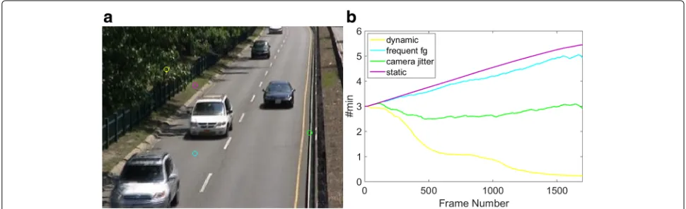
We usedN = 20 samples (Eq. (1)) to model the back-ground at each pixel location. The distance threshold parameterRfor determining match with the background model was set to 20. The parameterαin Eq. 2 was empiri-cally set to 19. This implies that #min decreases whenever the number of matches is less than 19. The parameterβin Eq. 2 controls the rate at which #min rises and decays and was empirically set to 2000. With these values, the maxi-mum that #min(x)can increase in a frame is by a factor of 1+1/2000=1.0005 (whennMatches(x)=20), while it can decrease by a factor of up to 1−18/2000 = 0.991 (whennMatches(x) = 1 and current #min(x) = 1 ). A fast decay and slow rise ensures that the algorithm read-ies itself quickly for dynamic conditions while it gauges the static nature only on long-term evidence. The initial value of 3 and an upper bound of 12 was set for #min. The value of #min will never become 0 by the recursive formula, so effectively the lower bound is 1. Although the adaptation results in fractional values for #min, the segmentation decision can change only when it crosses integer values. In other words, the effective value of #min is the current value rounded up to the next higher inte-ger. Figure 1 shows a frame from the baseline/highway video sequence of the CDnet dataset [7] and variation of #min for 4 sample pixels identified with colored cir-cles. For the pixel in dynamic background (yellow), #min falls below 1 by frame 900. The pixel on the crash bar-rier (green) experiences multiple modes due to camera jitter and #min stays around 3. For the pixel in the static area (magenta), #min increases smoothly and crosses 5 by the end of the sequence. For the pixel on the road (cyan), #min rises with fluctuations because the adaptation is fre-quently interrupted by the presence of vehicles. Note that these variations are also influenced by the spatial Gaussian smoothing which is applied every frame. Figure 2 shows the spatial distribution of #min for an example frame. It
can be seen that for dynamic regions, #min has been low-ered (darker regions). The effect of spatial smoothing of #min can also be noticed.
The parameters α and β were experimentally deter-mined to be 19 and 2000 considering various videos. For some categories of Cdnet dataset such as dynam-icBackground and cameraJitter, a slight improvement in F-measure was obtained with a smallerβof 1000 as #min adapted more quickly. However, the overall F-measure considering all categories was slightly lower. Values other than 19 forα resulted in lowerF-measure for almost all videos.
5 Proposed method: shadow detection
Our shadow detection method follows a two-stage approach and can detect achromatic as well as chro-matic shadows. Only pixels classified as foreground in the background subtraction step are considered as candidate shadow pixels because shadows labeled as background is not an issue in most applications. In the first stage, a weak shadow detector filters out impossible shadow values from the set of foreground pixels by imposing mild constraints on brightness, color distortion, and RGB values. Specifi-cally, for brightness, the input pixel is constrained to have a brightness less than the background pixel. For chroma, we adopted the color distortion measure in [24, 36] as they avoided the instability of normalized RGB. The threshold for allowed color distortion is intentionally permissive to include chromatic shadows as well. These tests on bright-ness and chroma lend nicely to our sample-based model. The input pixel should have brightness less than at least #min samples in the background model and the same sam-ples should be at a color distance less than a threshold with the input pixel. These two conditions alone tend to include dark objects as shadows since the color distortion between pixels is small near the origin of the RGB space. As noted in [27] and from our own analysis,R,G, andBvalues of a
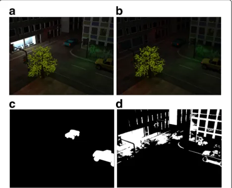
Fig. 2A frame from the dynamic background/ fountain01 video from CDnet and the spatial distribution of #min for the same frame
shadowed pixel are almost always above 20 (on a 0 to 255 scale), for all types of shadows. Therefore, this third con-dition is also incorporated in our initial shadow test (i.e., an input pixel should haveR,G, andBvalues above 20 to be considered as a shadow pixel). Foreground pixels sat-isfying these constraints on brightness, chroma, and RGB values result in a maskM1 on the current frame. Because of the liberal constraints, this initial maskM1 may contain some pixels from foreground objects, but this is taken care of in the second step. At this stage, it is important only that all shadow pixels are included inM1.
The second stage exploits the recurrence of similar shadow values at pixel level. A pixel-level shadow model is populated with actual shadowed pixel values. Collecting shadowed samples in a separate model for each pixel is an effective way to represent the change in pixel value when it comes under shadow. This shadow-induced variation in pixel value is otherwise highly difficult to character-ize because it depends on a huge number of factors such as nature and number of other light sources and reflec-tive properties of the surface as well as that of other scene objects and texture properties of the surface. However, since these factors which determine the shadow pixel val-ues are more or less stable, the valval-ues that a given pixel takes, when shadowed by different foreground objects, show a certain agreement even in complex illumination conditions [32]. Based on this rationale that shadow pixel values repeat at pixel level, each pixel in the initial shadow maskM1 is compared with the pixel-level shadow model and those pixels which find at least #min matches with the samples in the shadow model are labeled as shadow in the final shadow maskM2.
5.1 Shadow model initialization and maintenance
A problem in modeling shadows when compared to mod-eling background is that shadow appearance is not as frequent as background appearance. For our method to work properly, it has to be ensured that the shadow model contains enough shadow samples for matching and detec-tion. This is not an issue in busy highways and hallways where shadows appear frequently but has to be taken care
of in cases where foreground activity is rare. We address this issue in multiple ways. First, the shadow model is initialized directly from the background model by lin-early attenuating the RGB values of background samples. This readies the shadow model to detect achromatic shad-ows right from the first appearance. However, the scaling being linear, chromatic shadow pixels in mask M1 may not initially find matches with the shadow model, prevent-ing final shadow labelprevent-ing and update of shadow model. To avoid this deadlock situation, the shadow model is updated with the initial mask M1, without considering whether the pixel values are matched to the samples in the shadow model or not. This enables the shadow model to be filled with sufficient shadow samples for further match-ing. Of course, since the update maskM1 is based on test of brightness, color distortion, and RGB values only, it may cause some foreground values (which pass the weak detec-tor test based on these properties) also to be inserted in the model. But this is not troublesome as foreground val-ues are less likely to be repeated and matched than shadow values. The shadow model is updated with a higher prob-ability of 1/4, again due to the less frequent appearance of shadows compared to background.
5.2 Shadow detection parameters
Table 1SABS results:F-measures for various scenarios
Scenario Proposed Stauffer and Li et al. Zivkovic and van der Maddalena and Barnich and Haines and Xiang Grimson [42] [43] Heijden [13] Petrosino [35] Van Droogenbroeck [17] [14]
Basic 0.866 0.800 0.766 0.768 0.766 0.761 0.853
Dynamic 0.871 0.704 0.641 0.704 0.715 0.711 0.853
Bootstrap 0.765 0.642 0.678 0.632 0.495 0.685 0.796
Darkening 0.858 0.404 0.704 0.620 0.663 0.678 0.861
Light switch 0.459 0.217 0.316 0.300 0.213 0.268 0.603
Noisy night 0.733 0.194 0.047 0.321 0.263 0.271 0.788
Camouflage 0.813 0.802 0.768 0.820 0.793 0.741 0.864
No camouflage 0.879 0.826 0.803 0.829 0.811 0.799 0.867
H.264 (40 kbps) 0.893 0.761 0.773 0.748 0.772 0.774 0.827
Best values are italicized
6 Results and discussions
6.1 Background subtraction
The proposed method was implemented in MATLAB tak-ing advantage of its vectorization capabilities and tested on two popular public datasets: SABS [1] and CDnet [7]. For quantitative evaluation, we use F-measure as it is commonly considered to be the single best measure of performance. It is defined as the harmonic mean of recall and precision, where
recall=tp/(tp+fn), precision=tp/(tp+fp) (3)
Here,tpis the number of true positives (foreground),fp is the number of false positives, andfnis the number of false negatives.
The SABS dataset (available online [37]) consists of synthetic videos of a road junction simulating different real-world problems. They provide ground truth as well as evaluation code to generate performance metrics.Basic scenario combines many challenges for general perfor-mance evaluation.Dynamic backgroundscenario consid-ers the same sequence as basic but crops the test area to moving tree branches and a changing traffic light. Boot-strapscenario does not provide training frames without foreground objects.Darkeningscenario simulates gradual illumination decrease during sunset. Light switch sce-nario simulates sudden illumination change by switch-ing off a light and later turnswitch-ing it on again. In noisy night scenario, the sensor noise is high. In camouflage scenario, cars and people have colors similar to back-ground that they are hard to distinguish.H.264scenario video exhibits heavy compression artifacts. In Table 1, F-measure of our method is compared to that of other methods for various scenarios. Our method was tested on all scenarios with the same parameters (N = 20, R = 20, α = 19, β = 2000). Yet, the F-measure of the presented approach is close to the best performing method [14]. The light switch scenario is one of our weak
points as #min rises steadily till the switch is suddenly turned off. The sudden unexpected change in pixel val-ues results in massive false positive regions since only color values are used in our model. Figure 3 demon-strates this problem. Setting a lower upper bound for #min and increasing the distance threshold improves the results for this scenario, but this degrades recall in other scenarios.
The change detection dataset (available online [38]) is, by far, the largest dataset available. The 2012 CDnet dataset [7] contained nearly 90,000 frames in 31 video sequences grouped into 6 video categories. It was later expanded to 2014 CDnet dataset [39] by adding 22 more videos in 5 new categories. They provide hand-labeled ground truth maps for all frames and evaluation tools for generating the performance metrics. To allow for a
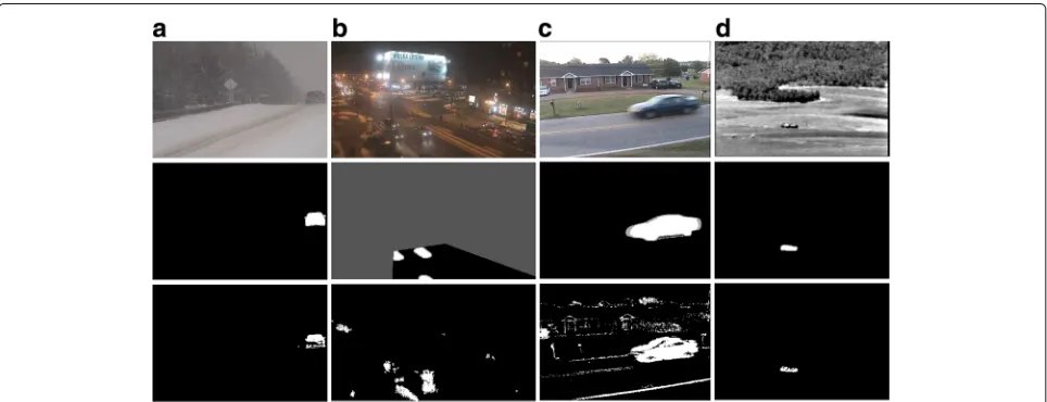
Fig. 4CDnet 2012 results typical detection results for 2012 CDnet dataset. On the first row is the input frame, on the second row is ground truth, and on the third row is background subtraction result of the presented method.aBaseline/office.bCamera jitter/badminton.cDynamic background/fall.dIntermittent object motion/sofa
model initialization period, the evaluation does not con-sider the results of the first few hundred frames. Our method was tested on the entire dataset and representa-tive segmentation results are shown in Figs. 4 and 5. To show how our method fares in comparison with alter-native methods, category-wiseF-measures are presented in Table 2. As shown in Table 2, a high F-measure is obtained for all categories in 2012 CDnet. The high F -measure fordynamic backgroundcategory demonstrates the effectiveness of adapting #min in combating dynamic background. The highF-measure forintermittent object motion category shows the effectiveness of our ghost
suppression mechanism. The overall F-measure of our method is higher than classic methods as well as simi-lar sample-based methods such as ViBe and PBAS which used more number of samples. F-measures for the new categories introduced in 2014 CDnet are lower since these categories are more difficult. The lowestF-measure score of 0.24 is obtained for PTZ category. This is not surprising as the basic assumption of static camera is violated in this category. Somewhat usable results for this category can be obtained by resorting to a blind update (updating both foreground and background pix-els). Varying the update rate based on camera movement
Table 2F-measures for 2012 CDnet
Method
Category Proposed KDE SC-SOBS ViBE PBAS CPDS DPGMM
(SBBS) [44] [45] [17] [19] [46] [14]
Baseline 0.919 0.909 0.933 0.870 0.924 0.921 0.929
dyn. background 0.813 0.596 0.669 0.565 0.683 0.750 0.814
Camera jitter 0.735 0.572 0.705 0.600 0.722 0.487 0.748
int. obj. motion 0.680 0.409 0.592 0.507 0.575 0.741 0.542
Shadow 0.711 0.803 0.779 0.803 0.860 0.809 0.813
Thermal 0.750 0.742 0.692 0.665 0.756 0.662 0.813
Overall 0.768 0.672 0.728 0.668 0.753 0.728 0.776
Best values are italicized
detection could be beneficial. The next lowestF-measure of 0.51 is for nightVideos category. This difficult cate-gory includes vehicular traffic videos captured at night. Color values are sharply varied by the effect of vehicle headlights. The road surface highlighted by the head-lights causes large non-vehicle foreground regions (see the second column of Fig. 5) and substantially deteriorates foreground extraction performance. To an extent, such spurious highlight detections can be eliminated by follow-ing an approach similar to shadow detection; that is, by utilizing the fact that highlights cast on the road surface
by different moving vehicles are similar and so pixel values repeat.
Other common performance metrics like recall, precision, specificity, false positive rate, false nega-tive rate, and percentage of wrong classification as well as complete segmentation results for various methods, including ours, are publicly available under Results tab on the changedetection.net website. All metrics were obtained by uploading the segmenta-tion results to the website and calculated using their software.
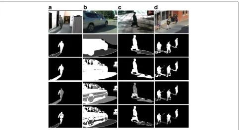
Fig. 7Shadow detection results for six benchmark sequences. On the first row is the input frame, on the second row is the ground truth, and the third row is the result of the presented shadow detection method. Shadow pixels are assigned a gray value of 127 in ground truth and in our result. aHighway I.bHighway II.cCampus.dLaboratory.eIntelligent room.fHallway
6.2 Shadow detection
The CDnet dataset contains a shadow category with two indoor and four outdoor videos. Hard shadows are labeled in the ground truth. For shadow detection per-formance evaluation, they define the False Positive Rate-Shadow (FPR-S) which is the ratio of the number of pixels labeled as shadow in ground truth but detected as foreground to the total number of pixels labeled as shadow in ground truth. However, popular shadow detection methods have not been tested on this dataset. The average FPR-S of 0.1228 of our method is the best of all methods tested on 2012 CDnet. Sample shadow
detection results for sequences from CDnet are shown in Fig. 6.
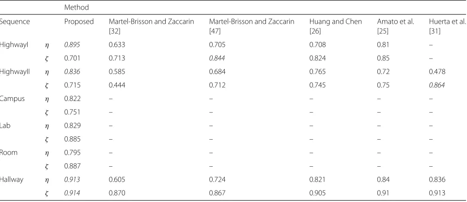
Commonly used sequences for benchmarking shadow detection algorithms are HighwayI,HighwayII, Campus, Laboratory, and Intelligent roomintroduced in [33] and Hallway introduced in [32]. HighwayI and HighwayII show traffic environments. In HighwayII, the shadows are chromatic. The Campus sequence is a noisy outdoor sequence. The lighting conditions and perspectives are different in the indoor sequences Lab and Room. In the Hallway sequence, multiple light sources are present and the floor is reflective. Qualitative results for these
Table 3Quantitative shadow detection results
Method
Sequence Proposed Martel-Brisson and Zaccarin Martel-Brisson and Zaccarin Huang and Chen Amato et al. Huerta et al.
[32] [47] [26] [25] [31]
HighwayI η 0.895 0.633 0.705 0.708 0.81 –
ζ 0.701 0.713 0.844 0.824 0.85 –
HighwayII η 0.836 0.585 0.684 0.765 0.72 0.478
ζ 0.715 0.444 0.712 0.745 0.75 0.864
Campus η 0.822 – – – – –
ζ 0.751 – – – – –
Lab η 0.829 – – – – –
ζ 0.885 – – – – –
Room η 0.795 – – – – –
ζ 0.887 – – – – –
Hallway η 0.913 0.605 0.724 0.821 0.84 0.836
ζ 0.914 0.870 0.867 0.905 0.91 0.913
sequences are presented in Fig. 7. The most commonly employed performance metrics are shadow detection rate (η) and shadow discrimination rate (ζ) introduced by Prati in [33]. These measures do not penalize shad-ows labeled as background or background labeled as shadow. Quantitative results comparing our method with other methods are presented in Table 3. Sequences and ground truth were taken from [40] and [41], and metrics were computed with all the available ground truth frames. Our detection rate is among the best for all sequences. This shows the suitability of our shadow detection method in detecting all types of shadows. The discrimination rate is somewhat low for HighwayI and HighwayII because of the repeated appearance of severely shadow-camouflaged vehicle parts, windscreens in par-ticular (see columns 1 and 2 in Fig. 7). Better results or trade-off between detection rate and discrimination rate could be obtained by hand tuning the parameters (scaling factor for initializing shadow model from background model, color distance threshold, RGB values threshold, distance threshold and required number of matches for comparison with shadow model, update rate) for each sequence.
6.3 Computational cost
The speed advantage of sample-based methods compared to parametric methods like GMM has been reported in [17]. Compared to ViBe [17], the proposed method offers a speed advantage which stems from the fact that L1 distances are used whereas [17] used L2 distances. Com-pared to (PBAS) [19], the proposed method uses fewer samples (35 vs 20) and hence lesser computational cost while still obtaining a better performance. Compared to SuBSENSE [20], which uses 50 samples per pixel, our method uses only 40 samples for combined background subtraction and shadow detection, resulting in a lower overall computational complexity. In addition, the pro-posed method has fewer parameters compared to PBAS and SuBSENSE which also helps in reducing the compu-tational complexity.
7 Conclusion
Sample-based modeling has proven to outperform con-ventional methods of background modeling. The pre-sented method addressed the issue of under-utilization of samples in stable regions of the background with continuous per-pixel adaptation of the number of matches required to classify a pixel as background. Experimen-tal results have proven the robustness of our method in various scenarios. Shadow detection which was often done independently of background subtraction is inte-grated in our approach. Our novel approach of populating the shadow model with actually observed shadow pixel values solves the difficult problem of modeling different
types of shadows. As shown by experimental results, our two-stage shadow detector can accurately model and reli-ably detect shadows, no matter what the illumination condition, geometry or texture of the background, and orientation or type of shadow are. Since both background and shadow models are at pixel level and employ only pixel values with few parameters, our combined back-ground subtraction and shadow detection algorithm are well suited for fast hardware implementations.
Acknowledgements
The authors would like to thank all the people associated with the research lab of NIT Calicut for providing the facilities needed.
Funding None.
Authors’ contributions
Both authors contributed equally for this work. AV designed and performed the experiments. SG supervised the work and contributed to the writing of the paper. Both authors read and approved the final manuscript.
Competing interests
The authors declare that they have no competing interests.
Publisher’s Note
Springer Nature remains neutral with regard to jurisdictional claims in published maps and institutional affiliations.
Received: 25 May 2017 Accepted: 7 December 2017
References
1. Brutzer S, Hoferlin B, Heidemann G (2011) Evaluation of background subtraction techniques for video surveillance. In: Computer Vision and Pattern Recognition (CVPR), 2011 IEEE Conference On. IEEE. pp 1937–1944 2. Piccardi M (2004) Background subtraction techniques: a review. In:
Systems, Man and Cybernetics, 2004 IEEE International Conference On, vol. 4. IEEE. pp 3099–3104
3. Radke RJ, Andra S, Al-Kofahi O, Roysam B (2005) Image change detection algorithms: a systematic survey. Image Proc IEEE Trans 14(3):294–307 4. Bouwmans T, El Baf F, Vachon B (2008) Background modeling using
mixture of Gaussians for foreground detection—a survey. Recent Patents Comput Sci 1(3):219–237
5. Bouwmans T (2014) Traditional and recent approaches in background modeling for foreground detection: an overview. Comput Sci Rev 11:31–66
6. Sobral A, Vacavant A (2014) A comprehensive review of background subtraction algorithms evaluated with synthetic and real videos. Comp Vision Image Underst 122:4–21
7. Goyette N, Jodoin PM, Porikli F, Konrad J, Ishwar P (2014) A novel video dataset for change detection benchmarking. Image Process IEEE Trans 23(11):4663–4679
8. Wren CR, Azarbayejani A, Darrell T, Pentland AP (1997) Pfinder: real-time tracking of the human body. Pattern Anal Mach Intell IEEE Trans 19(7):780–785
9. Stauffer C, Grimson WEL (2000) Learning patterns of activity using real-time tracking. Pattern Anal Mach Intell IEEE Trans 22(8):747–757 10. Power PW, Schoonees JA (2002) Understanding background mixture
models for foreground segmentation. In: Proceedings Image and Vision Computing New Zealand, vol. 2002. pp 10–11
11. KaewTraKulPong P, Bowden R (2002) An improved adaptive background mixture model for real-time tracking with shadow detection. In: Video-based Surveillance Systems. Springer. pp 135–144
13. Zivkovic Z, van der Heijden F (2006) Efficient adaptive density estimation per image pixel for the task of background subtraction. Pattern Recogn Lett 27(7):773–780
14. Haines TS, Xiang T (2014) Background subtraction with Dirichlet process mixture models. Pattern Anal Mach Intell IEEE Trans 36(4):670–683 15. Elgammal A, Duraiswami R, Harwood D, Davis LS (2002) Background and
foreground modeling using nonparametric kernel density estimation for visual surveillance. Proc IEEE 90(7):1151–1163
16. Mittal A, Paragios N (2004) Motion-based background subtraction using adaptive kernel density estimation. In: Computer Vision and Pattern Recognition, 2004. CVPR 2004. Proceedings of the 2004 IEEE Computer Society Conference On, vol. 2. IEEE. p 302
17. Barnich O, Van Droogenbroeck M (2011) Vibe: a universal background subtraction algorithm for video sequences. Image Process IEEE Trans 20(6):1709–1724
18. Wang H, Suter D (2007) A consensus-based method for tracking: modelling background scenario and foreground appearance. Pattern Recog 40(3):1091–1105
19. Hofmann M, Tiefenbacher P, Rigoll G (2012) Background segmentation with feedback: the pixel-based adaptive segmenter. In: Computer Vision and Pattern Recognition Workshops (CVPRW), 2012 IEEE Computer Society Conference On. IEEE. pp 38–43
20. St-Charles PL, Bilodeau GA, Bergevin R (2015) Subsense: a universal change detection method with local adaptive sensitivity. Image Process IEEE Trans 24(1):359–373
21. Cucchiara R, Grana C, Piccardi M, Prati A (2003) Detecting moving objects, ghosts, and shadows in video streams. Pattern Anal Mach Intell IEEE Trans 25(10):1337–1342
22. Schreer O, Feldmann I, Gölz U, Kauff P (2002) Fast and robust shadow detection in video conference applications. In: Video/Image Processing and Multimedia Communications 4th EURASIP-IEEE Region 8 International Symposium on VIPromCom. IEEE. pp 371–375 23. Cavallaro A, Salvador E, Ebrahimi T (2005) Shadow-aware object-based
video processing. In: Vision, Image and Signal Processing, IEE Proceedings-, vol. 152. IET. pp 398–406
24. Horprasert T, Harwood D, Davis LS (1999) A statistical approach for real-time robust background subtraction and shadow detection. In: IEEE ICCV, vol. 99. pp 1–19
25. Amato A, Mozerov MG, Bagdanov AD, Gonzalez J (2011) Accurate moving cast shadow suppression based on local color constancy detection. Image Process IEEE Trans 20(10):2954–2966
26. Huang JB, Chen CS (2009) Moving cast shadow detection using physics-based features. In: Computer Vision and Pattern Recognition, 2009. CVPR 2009. IEEE Conference On. IEEE. pp 2310–2317 27. Salvador E, Cavallaro A, Ebrahimi T (2004) Cast shadow segmentation
using invariant color features. Comp Vision Image Underst 95(2):238–259 28. Nadimi S, Bhanu B (2004) Physical models for moving shadow and object detection in video. Pattern Anal Mach Intell IEEE Trans 26(8):1079–1087 29. Yao J, Odobez JM (2007) Multi-layer background subtraction based on
color and texture. In: Computer Vision and Pattern Recognition, 2007. CVPR’07. IEEE Conference On. IEEE. pp 1–8
30. Leone A, Distante C (2007) Shadow detection for moving objects based on texture analysis. Pattern Recog 40(4):1222–1233
31. Huerta I, Holte MB, Moeslund TB, Gonzàlez J (2015) Chromatic shadow detection and tracking for moving foreground segmentation. Image Vision Comput 41:42–53
32. Martel-Brisson N, Zaccarin A (2007) Learning and removing cast shadows through a multidistribution approach. Pattern Anal Mach Intell IEEE Trans 29(7):1133–1146
33. Prati A, Mikic I, Trivedi MM, Cucchiara R (2003) Detecting moving shadows: algorithms and evaluation. Pattern Anal Mach Intell IEEE Trans 25(7):918–923
34. Sanin A, Sanderson C, Lovell BC (2012) Shadow detection: a survey and comparative evaluation of recent methods. Pattern Recogn
45(4):1684–1695
35. Maddalena L, Petrosino A (2008) A self-organizing approach to background subtraction for visual surveillance applications. Image Process IEEE Trans 17(7):1168–1177
36. Kim K, Chalidabhongse TH, Harwood D, Davis L (2005) Real-time foreground–background segmentation using codebook model. Real-Time Imaging 11(3):172–185
37. SABS Dataset. http://www.vis.uni-stuttgart.de/index.php?id=sabs 38. CDnet Dataset. http://www.changedetection.net
39. Wang Y, Jodoin PM, Porikli F, Konrad J, Benezeth Y, Ishwar P (2014) Cdnet 2014: an expanded change detection benchmark dataset. In: Proceedings of the IEEE Conference on Computer Vision and Pattern Recognition Workshops. pp 387–394
40. Shadow detection sequences and ground truth. http://vision.gel.ulaval. ca/~CastShadows/
41. Shadow detection sequences and ground truth. http://arma.sourceforge. net/shadows/
42. Stauffer C, Grimson WEL (1999) Adaptive background mixture models for real-time tracking. In: Computer Vision and Pattern Recognition, 1999. IEEE Computer Society Conference On, vol. 2. IEEE
43. Li L, Huang W, Gu IY, Tian Q (2003) Foreground object detection from videos containing complex background. In: Proceedings of the Eleventh ACM International Conference on Multimedia. ACM. pp 2–10 44. Elgammal A, Harwood D, Davis L (2000) Non-parametric model for
background subtraction. In: Computer Vision—ECCV 2000. Springer. pp 751–767
45. Maddalena L, Petrosino A (2012) The sobs algorithm: what are the limits? In: Computer Vision and Pattern Recognition Workshops (CVPRW), 2012 IEEE Computer Society Conference On. IEEE. pp 21–26
46. Hernandez-Lopez FJ, Rivera M (2014) Change detection by probabilistic segmentation from monocular view. Mach Vis Appl 25(5):1175–1195 47. Martel-Brisson N, Zaccarin A (2008) Kernel-based learning of cast shadows