Modeling Users’ Behavior from Large Scale
Smartphone Data Collection
Preeti Bhargava
1,∗, Ashok Agrawala
11Department of Computer Science, University of Maryland, College Park, MD, USA
Abstract
A large volume of research in ubiquitous systems has been devoted to using data, that has been sensed from users’ smartphones, to infer their current high level context and activities. However, mining users’ diverse longitudinal behavioral patterns, which can enable exciting new context-aware applications, has not received much attention. In this paper, we focus on learning and identifying such behavioral patterns from large-scale data collected from users’ smartphones. To this end, we develop a unified infrastructure and implement several novel approaches for building diverse behavioral models of users. Examples of generated models include classifying users’ semantic places and predicting their availability for accepting calls etc. We evaluate our work on real-world data of 200 users, from the DeviceAnalyzer dataset, consisting of 365 million data points and show that our algorithms and approaches can model user behavior with high accuracy and outperform existing approaches.
Receivedon 8 May 2016;acceptedon 21 June 2016;publishedon 12 September 2016
Keywords: Context-aware computing and systems, User behavior modeling, Learning from context
Copyright © 2016 P. Bhargava and A. Agrawala, licensed to EAI. This is an open access article distributed under the terms oftheCreativeCommonsAttributionlicense(http://creativecommons.org/licenses/by/3.0/),whichpermits unlimiteduse,distributionandreproductioninanymediumsolongastheoriginalworkisproperlycited.
doi:10.4108/eai.12-9-2016.151677
1. Introduction
While discrete observations of an individual’s behavior can appear almost random, typically there are repet-itive and easily identifiable patterns or routines in every person’s life. For many people, a typical weekday routine consists of leaving home in the morning and traveling to work, going for lunch in the afternoon, and returning home in the evening. These daily routines are often coupled with routines across other temporal scales, such as weekly (e.g. going hiking or running on weekends) or monthly (e.g. visiting family during holidays) patterns.
In today’s world, smartphones are the most ubiqui-tous devices and have become an integral part of peo-ple’s everyday lives. People carry them around every-where and use them as their primary medium for many day to day activities. These devices can collect a variety of data about users such as their locations (from GPS), sensory data (from various sensors), call and sms logs etc. As a result, they can act as a rich content source for users’ contextual information. However, a large volume
∗
Corresponding author. Email:[email protected]
of research in mobile and ubiquitous systems has been devoted to using this collected information for inferring users’ current high level context such as their environ-mental context (whether they are indoors or outdoors), the activities they are engaged in (walking, driving etc.) and how many people are around them [5,20,21]. On the other hand, mining of users’ diverse longitudinal behavioral patterns from rich smartphone data, which can enable exciting new context-aware applications and services, has not received much attention.
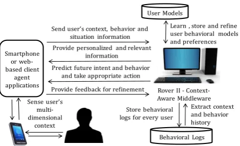
Figure 1 shows our broader long-term vision. As part of this vision, we plan to collect large-scale data from users’ smartphones and employ it to infer diverse frequent patterns that capture different aspects of their behavior. We plan to explore the utility of each type of pattern in improving the users’ quality of life by proactively taking actions on their behalf. As shown, we envision a client agent application continuously sensing the user’s temporal multi-dimensional context and activity information (e.g. location, call logs and app usage). This information is aggregated over a period of time in the form of behavioral logs. A context-aware middleware extracts the user’s context history
(for instance, call or location history) from these logs.
It utilizes this history to learn and store the users’
behavioral models(behavioral patterns that users exhibit in similar context or situations over a period of time) for predicting future behavior. Ultimately, this enables the middleware to act proactively on the users’ behalf in anticipation of their future goals and intentions without explicit requests from them. The system also refines these models periodically based on users’ feedback.
In this paper, we take a step towards achieving this vision. We develop an infrastructure for learning diverse patterns, from large-scale data collected from users’ smartphones, and utilizing these patterns to help identify a variety of the users’ behaviors, habits, and daily life places and activities. A key aspect of our research is how to mine this massive amount of data, captured over long durations of time, for inferring users’ high level behavioral models. In particular, we try to answer questions such as:
• What are the various places frequently visited by the user? Which among them is his home, workplace, recreational or known places etc.?
• Will the user accept an incoming call in his current situation? Who will be the next person that he will call?
• When and where does the user usually charge his device? How is his device battery usage and can we predict his future device battery level?
• What applications (referred to as ‘apps’) does he use most frequently in the morning as opposed to night?
These behavioral models would enable the context-aware system to predict a user’s behavior and proactively take actions on his behalf. For instance, the system can leverage a user’s past communication behavior in order to predict his availability to accept an incoming call and proactively reject it if he is unavailable (say, if he is in a meeting at work). It could periodically order the user’s contacts based on who will be the most likely contact that will be called next. Similarly, it can employ his device charging behavior to prompt him if he forgets to charge his device. It can even load his favorite apps ahead of time based on his app usage history. Ultimately, such a system can save the user’s time and energy and improve his quality of life.
Our key contributions in this paper are:
• We design and implement a unified infrastructure for modeling a diverse set of users’ behaviors from large-scale data that has been collected from their smartphones.
• We design and implement novel approaches and algorithms that employ users’ contextual features
Smartphone or web-based client
agent applications
Rover II - Context-Aware Middleware Predict future intent and behavior
and take appropriate action Send user’s context, behavior and
situation information
Provide feedback for refinement
Store behavioral logs for every user
Extract context and behavior history
Behavioral Logs User Models
Learn , store and refine user behavioral models and preferences
Sense user’s multi-dimensional
context
Provide personalized and relevant information
Figure 1. Long term vision for building diverse user behavioral models, from users’ sensed data, in order to take proactive actions
and state of the art machine learning techniques for building various behavioral models of users. Examples of generated models include classifying users’ semantic places (such as Home, Work etc.) and mobility states (Stationary or Moving), pre-dicting their availability for accepting incoming calls and inferring their device charging behavior.
• We evaluate our work on large-scale real-world smartphone data of 200 users, obtained primarily from the DeviceAnalyzer[28] dataset, consisting of 365 million data points.
• We show that our algorithms and approaches can model user behavior with high accuracy and demonstrate improved performance over existing approaches.
2. Rover II context-aware
middleware
The Rover II context-aware middleware [6, 17] is a generic middleware, which serves as an integration platform for mobile and desktop applications. It can store and retrieve contextual information, as well as learn and store user behavior models. It consists of several components including a main Controller module (which controls the flow of information among the various components), an Activity Manager (which defines what activities the system can perform on the user’s behalf), a Learning Engine (which learns patterns from user’s behavior) and a Relevant Information Discovery and Ranking Engine (which determines what information will be relevant to the user’s current situation). A complete description of this system and its architecture is beyond the scope of this paper. Here, we describe the core component responsible for learning user behavioral models - the Learning Engine.
User behavioral
logs
Log Query Module Context
history
<User1, t1, Location, <latitude, longitude>> <User1, t2, Call|Number, Number hash> <User1, t2, Call|Duration, Call duration in seconds>
……… Learning Engine
User behavioral models
kNN Naïve Bayes J48 SMO Random
Forest
HMM
kMeans Apriori PredictiveApriori
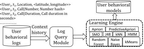
Figure 2. The Learning Engine pipeline of Rover II
smartphone and stored in a relational database in the form of timestamped <key,value> pairs where each key is unique and represents the type of contextual data that is logged and the value represents the value for that contextual data e.g. location (represented in latitude and longitude format) or call data such as number called, duration etc. The data is stored in chronological order. The Log Query Module extracts the user’s context history (location trace, sensor log, call history etc.) over a certain window of time, from these logs, and sends it to the Learning Engine.
The Learning Engine implements several state of the art supervised and unsupervised machine learning techniques including classifiers such as J48 Decision Tree,kNearest Neighbors (kNN), Naive Bayes, Random Forest, and Sequential Minimal Optimization (SMO) [24] (an algorithm used for training support vector machines), clustering algorithms such as kMeans and DBSCAN, association rule mining algorithms such as Apriori and PredictiveApriori as well as Hidden Markov Models (HMM) that model causal relationships. In the current version of our system, we employ the Weka[12] and ELKI [1] libraries for implementing these techniques.
The engine extracts various contextual features from the users’ context history and applies these techniques to them in order to generate user behavior models. These models are either held in memory for immediate use or persisted to disk for subsequent usage in prediction of users’ behavior.
3. Data
The data used in this research comes from two sources:
3.1. DeviceAnalyzer dataset
DeviceAnalyzer [28] is a free smartphone based Android application that runs continuously in the background and collects a user’s data from his smartphone. It was developed to collect a large-scale research data-set of phone usage. It has collected usage information from 17,000 Android devices, over the course of nearly 3 years, and contains 100 billion data points. It captures a rich and highly detailed time-series
log of approximately 300 different events1 including sensory information, Wi-Fi and bluetooth scans, call and sms logs, running processes and applications etc. This data is stored in the form of timestamped key-value pairs.
Since not all users in the DeviceAnalyzer dataset consented to sharing location and sensory information, we pre-processed the data to include only those users who have shared all information from their phone. In order to have enough training and testing instances, we also set the criteria that only those users who have > 30 days of data should be included. Our final dataset consists of 200 users and includes over 365 million data points logged over 100,000 days for all users. We use about 20% of this data as Validation data for parameter tuning.
3.2. Field study
Despite the richness of the DeviceAnalyzer dataset, a disadvantage of it is that it does not have ground truth labels for semantic places and for mobility states. To address this, we conducted a field study using the DeviceAnalyzer app to collect labeled data over a period of 1 month. This data was collected by 10 members of our lab (including the first author). All the participants who collected the data also annotated it carefully to provide ground truth values for place labels (see Table 4) and mobility states (see Table 2). This dataset consisted of around 500,000 data points. We split this dataset into Training and Testing data with a 1:1 ratio. We used the training dataset for building some of the models and the testing set for their evaluation.
4. Feature engineering and Algorithm Design for
User behavior modeling
4.1. Mobility State Classification
The DeviceAnalyzer app samples the data from the accelerometer of a device at a frequency of approxi-mately 0.003 Hz (once per 5 minutes). Moreover, this data is not logged in its raw format but as aggre-gate measurements (such as count, variance, average etc.) computed over all magnitudes of sensor values captured over a 1-second window. Hence, fine-grained activity recognition as performed in [5,20,21] is not possible with this dataset.
Instead, we use this data to classify the user’smobility state into two classes - Stationary and Moving. We extract movement related features such as average and variance of acceleration (see Table 1) to build this model. We experimented with 3 classifiers - kNN
Feature Description or Representa-tion
Average acceleration
Average acceleration of the device
Variance of acceler-ation
Variance of acceleration of the device
Table 1. Movement related features
Label Description or
Representa-tion
Stationary Whether user is stationary
Moving Whether user is moving
Table 2. Mobility state labels
Accuracy kNN J48 Random Forest
0.81 0.72 0.85
Table 3. Comparison of accuracies of various classifiers on the training set for Mobility State Classification
(k=3), Random Forest (10 trees) and J48 decision tree on the training data collected as part of the field study (see Section 3.2) with 10 fold cross validation. As shown in Table 3, Random Forest had the best performance. Hence, we implement it for Mobility State Classification.
4.2. Timestamp hashing
Since the number of timestamps in our dataset is huge (as it spans nearly 100,000 days of data for all users), we perform feature hashing to hash the value of each timestamp to a timeslot in order to reduce the data dimensionality. We generate buckets of hashed time slots based on the day of the week and time of the day. This also enables us to capture daily and hourly patterns in behavior which further help in user behavior modeling.
To this end, we divide a day into 4 hourly slots:
• Morning - hours between 5 am and 10 am
• Noon - hours between 10 am and 5 pm
• Evening - hours between 5 pm and 10 pm
• Night - hours between 10 pm and 5 am
We generated these slots using commonsense knowl-edge that most people tend to share common daily patterns - they typically sleep between 10 pm and 5 am, commute between 8 and 9 am and reach work between 9 and 10 am. In addition, most places have work hours till 4:30 or 5 pm.
Since there are 2 types of days in a week - weekday and weekend, and each day has 4 hourly slots, the total number of hashed timeslots is 8. Each timestamp is first
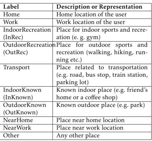
Label Description or Representation
Home Home location of the user
Work Work location of the user
IndoorRecreation (InRec)
Place for indoor sports and recre-ation (e. g. gym)
OutdoorRecreation (OutRec)
Place for outdoor sports and recreation (walking, hiking, run-ning etc.)
Transport Place related to transportation
(e.g. road, bus stop, train station, parking lot)
IndoorKnown (InKnown)
Known indoor place (e.g. friend’s home or a coffee shop)
OutdoorKnown (OutKnown)
Known outdoor place (e.g. park)
NearHome Place near home location
NearWork Place near work location
Other Any other place
Table 4. Semantic place class labels
converted to a standard date time format which is then hashed to a timeslot. For instance, a timestamp of 2013-05-17 14:07:00 will be hashed to ‘WeekDay_Noon’.
4.3. Semantic Place Classification
Semantic Place Classification involves association of appropriate meaningful semantic labels with a user’s location2. Knowing the semantics of a location can enable a context-aware system to provide the user with information relevant to his current location e.g. work related notes at work or grocery list when he is at the grocery store. Moreover, this knowledge can also help predict other behaviors of the user such as his availability to attend a call or his intention to charge his phone.
As mentioned earlier, human behavior usually follows a regular pattern in practice e.g. people sleep at home at night, move continuously when in the gym or running outside, and charge their phones indoors. We exploit these patterns to label the semantic places of users. Table 4 shows the 10 semantic place labels which we use to classify the locations in a user’s location history. Some of these overlap with those used in the Nokia Mobile Data Challenge (MDC) dataset [16,18].
The location data in the DeviceAnalyzer dataset has been obtained via the Android network provider, instead of GPS, due to privacy constraints. The network provider determines user location via cell tower and Wi-Fi signals. As a result, the obtained location is coarse-grained and not very accurate. Moreover,
Feature Description or Representation
Place visit count Number of unique visits to a place
Relative place
visit frequency
Number of visits (per day) to a place
Place stay dura-tion
Total stay duration at each place
Average place
stay duration
Average stay duration (per visit) at each place
Place - Time slot visit frequency
Number of unique time slots for each visited place
Time slot - place visit frequency
Place visit count for each time slot
Time slot - place time frequency
Place stay time for each time slot
Bluetooth count Average number of people
around at each place Bluetooth
diver-sity
Change in the people for consec-utive visits to each place
Wi-Fi count Average number of unique
Wi-Fi APs heard at each place
Wi-Fi RSSI Average Wi-Fi RSSI at each
place Wi-Fi
connectiv-ity
Wi-Fi connectivity status at each place
Charging state
frequency
Charging state of the device at each place - connected (via ac/usb) or disconnected
Mobility state
frequency
Mobility state of the device at each place - stationary or moving
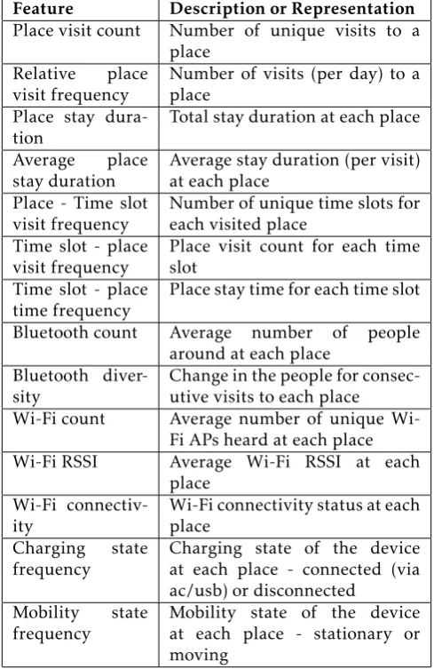
Table 5. Spatial and temporal features used for Semantic Place Classification
location sampling is duty cycled to conserve power. Hence, we rely on several additional features to label a user’s locations. Table 5 shows the 14 spatial and temporal features that we extract from a user’s context history and employ for semantic place classification. These are:
• Place visit count: This is computed as the number of unique visits to a place. This feature helps in identifying places such as ‘Home’ which a user would visit the most.
• Relative place visit frequency: This is the number of visits to a place per day and is computed as
Number of unique visits to a place
Total number of days in the user’s location history
This feature too helps in identifying places such as ‘Home’ which would be visited almost everyday.
• Place stay duration: This is computed as the total time spent at a place. This again should be high for ‘Home’ as most people spend a bulk of their day at home.
• Average place stay duration: This is the average stay duration at a place (per visit) and is computed as
Total stay duration at a place Number of visits to the place .
• Place - Time slot visit frequency: This is computed by counting the unique time slots at which a place has been visited by the user. This feature helps in identifying places such as ‘Home’ and ‘Work’ as most people visit their homes at all possible time slots but usually visit their work place on weekdays only.
• Time slot - place visit frequency: This is computed by calculating the count of a user’s unique visits to a place in each time slot.
• Time slot - place time frequency: This is computed by calculating the total time spent at a place, by the user, in each time slot. These temporal features too help identify ‘Home’ and ‘Work’ as most people are at home during the night and at work during the noon time slots.
• Bluetooth count: As suggested by our previous work in [5], bluetooth count can be utilized to determine the number of people around. We compute an average bluetooth count for each unique place in the user’s location history.
• Bluetooth diversity: To compute this, we deter-mine the set of bluetooth devices scanned at each unique visit to a place. For every two consecutive visits, we compute the ratio of the intersection to the union of the device sets and average all the values to generate a final value. The bluetooth features are useful for identifying places such as recreational spots which several people may visit and at different times.
• Wi-Fi count: This is computed by counting the number of visible Wi-Fi Access Points (APs) heard at a location for each unique visit and averaging the values.
• Wi-Fi connectivity status: This is generated as the count of times the user’s device is connected to Wi-Fi at a place. This feature helps in identifying places that are known to a user as his/her device would connect to the Wi-Fi network at a known place only and if it has access to it.
• Charging state frequency: This represents the charging state (ac, usb or disconnected) frequen-cies of the device at a place. This feature too helps in distinguishing between indoor and outdoor environments as ac charging can occur indoors only.
• Mobility state frequency: This represents the mobility state (stationary/moving) frequencies of the user at a place. This feature helps identify recreational and transportation places where the user would exhibit more movement.
The Learning Engine of Rover II employs Algorithm 1 for identifying the semantic labels of all the places visited by a user. The algorithm takes as input the user’s context history consisting of the 14 spatial and temporal features described in Table 5. It returns the list of all locations, as well as their semantic place labels, in the user’s location history.
As shown, we first hash each timestamp in the user’s context history to a time slot. We then discretize each location (expressed in latitude and longitude), in the user’s location history, into virtual rectangular bins that are formed throughout the geographical coordinate space. This helps in reducing redundancy in the locations. Each bin is created through a location hashing function which takes as input: (i) latitude and longitude as 64-bit floats and (ii) a bin size r in meters. The function leverages the fact that latitude and longitude are expressed in decimal degrees, with the fifth decimal place corresponding roughly to 1 meter. Since this precision was acceptable to us, we truncated each value to five decimal places. The function produces the resulting integer key with the longitude and latitude ending up in the high and low bits, respectively. This key identifies a virtual bin approximatelyrmeters per side, although the bin will be elongated north-to-south for regions further away from the equator due to the Earth’s curvature. Based on empirical observations, we setras 500m in our current implementation.
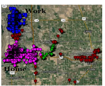
We then cluster the hashed locations using the DBSCAN [9] algorithm which identifies clusters in large spatial datasets by looking at the local density of database elements. DBSCAN takes two parameters as input - MinPts which is the minimum number of points in the vicinity of a point in order for it to be the cluster center andEpswhich is the vicinity radius. We setMinPtsas 100 andEpsas 2400m in our current implementation. Figure 3 show the location clusters
Figure 3. Location clusters for a randomly chosen user in our dataset (best viewed in color).
generated for a randomly chosen user in our dataset. To improve legibility of the figure, so that individual locations can be discerned, we sampled the number of data points down. The user’s ‘Home’ cluster (colored in pink) and the ‘Work’ cluster (colored in blue) are clearly evident. The locations colored in maroon are outliers or ‘Noise’ as determined by DBSCAN as they do not belong to a cluster but are other places that are visited by the user.
We now extract the spatial and temporal features described earlier, for each hashed location, and use them for labeling the locations. We first identify the user’s ‘Home’ location. To achieve this, we exploit the fact that ‘Home’ is the place where we spend the most time, which we visit the most and on all days and at all possible time slots. Once the ‘Home’ is obtained, we identify his ‘Work’ location. Most people follow a day time schedule and hence we classify ‘Work’ as the place which is not ‘Home’, and which is visited most and where most time is spent during the noon time slot. We also utilize the fact that ‘Work’ will usually not be visited on weekends (hence, ratio of time spent on weekends to weekdays will be< 1) and will not be visited at all possible time slots.
Algorithm 1:Algorithm for Semantic Place Classification
Input: User’s context history data consisting of the spatial and temporal features described in Table5
Output: List of locations visited by user and their semantic place labels
foreachTimestamp for which there is a location loggeddo
Hash each timestamp to a time slot;
Hash each location (in latitude and longitude format) to a discrete virtual rectangular bin of size 500m;
end
Cluster the hashed locations using DBSCAN based on distance;
// Extract the spatial and temporal features
foreachhashed location in user’s location historydo
Compute the total stay duration, visit count, time slot - place visit frequency, average stay duration and relative visit frequency;
Compute the time slot at which the location is visited most and the count of unique time slots at which it is visited;
Compute the ratio of time spent on weekends to time spent on weekdays for the location; Compute the average count of visible Wi-Fi APs and the average Wi-Fi RSSI for the location; Compute the average count and diversity of bluetooth devices for the location;
Compute the normalized mobility state frequencies, charging state frequencies and Wi-Fi connectivity status for the location;
end
foreachtime slotdo
Compute the total place stay duration and place visit counts for each visited place, in the user’s location history, for the time slot;
Compute the location that is visited the most, and the location at which the most time is spent most, during this time slot;
end
// Label ‘Home’ and ‘Work’
Label ‘Home’ as the location that has the highest stay duration, highest relative visit frequency, highest visit count and has been visited at all time slots;
Label ‘Work’ as the place that is visited most or where most time is spent during the Noon time slot, which is not ‘Home’, for which the ratio of weekend to weekday time<1.0 and which has not been visited on all time slots;
// Label other places
foreachhashed location in user’s location history (other than ‘Home’ and ‘Work’)do
Label as ‘IndoorRecreation’, ‘OutdoorRecreation’ or ‘Transport’ based on its features such as normalized mobility state of the user, average count of visible Wi-Fi APs, average Wi-Fi RSSI, average bluetooth count and diversity ;
end
foreachunlabeled hashed location in user’s location historydo
Label as ‘IndoorKnown’ or ‘OutdoorKnown’ based on features such as visit count, # of time slots at which visited, average count of visible Wi-Fi APs, average Wi-Fi RSSI, and Wi - Fi connectivity status;
iflocation not labeled as ‘IndoorKnown’ or ‘OutdoorKnown’then iflocation belongs to the same cluster as Homethen
Label as ‘NearHome’;
else iflocation belongs to the same cluster as Workthen
Label as ‘NearWork’;
else
Label as ‘Other’;
end
returnList of locations visited by user and their semantic place labels;
Locations which do not get classified into these 3 classes are then categorized as ‘IndoorKnown’ and ‘OutdoorKnown’ based on features such as their visit
Accuracy kNN J48 Naive Bayes
0.78 0.85 0.63
Table 6. Comparison of accuracies of various classifiers on the training set for Semantic Place Classification
Feature Description or Representation
Hashed time
slot
Time of day and Day of week at the time of the call
Semantic Place
Semantic location of the user (Home/Work/Transport etc.) Bluetooth
count
Number of people around
Mobility state Whether user is moving or sta-tionary
Average call frequency
Average number of calls made (per hour) during each time slot Average ring
frequency
Average number of calls received (per hour) during each time slot Average
missed call
frequency
Average number of calls missed (per hour) during each time slot
Average
missed call
rate
% of the calls received that are missed during each time slot
Average call duration
Average call duration during a time slot
Average
call time
difference
Average time difference (in min-utes) between calls made during a time slot
Average
ring time
difference
Average time difference (in min-utes) between calls received dur-ing a time slot
Average SMS
out frequency
Average number of SMS sent (per hour) during a time slot
Average SMS
in frequency
Average number of SMS received (per hour) during a time slot Table 7. Spatial and temporal features used for call acceptance prediction
device. This approach is also intuitive as known places (such as a friend’s home or a coffee shop) will be visited more often by the user and possibly at different times of day. Moreover, a user’s device will be connected to Wi-Fi at a known place that he would have visited before. Finally, places which do not fall into the ‘Known’ class are then classified based on the clusters they belong to. All unlabeled places in the ‘Home’ cluster of a user are labeled as ‘NearHome’ and all places in the ‘Work’ cluster are labeled as ‘NearWork’. Finally, all remaining unlabeled places are labeled as ‘Other’.
We experimented with kNN (k=3), J48 decision tree and Naive Bayes classifiers for classifying the places into the 8 classes as mentioned above. Table 6 shows
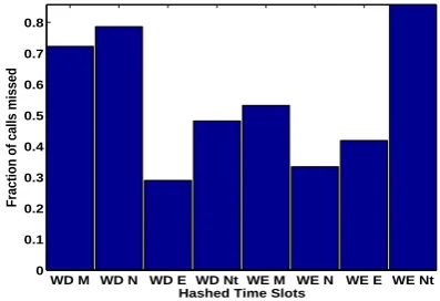
WD M WD N WD E WD Nt WE M WE N WE E WE Nt 0
0.1 0.2 0.3 0.4 0.5 0.6 0.7 0.8
Hashed Time Slots
Fraction of calls missed
Figure 4. % of calls missed in different time slots for a randomly chosen user from our dataset
the accuracies for these 3 classifiers on the training data collected as part of the field study (see Section3.2) with 10 fold cross validation. J48 had a superior performance and faster training time than kNN and Naive Bayes. Hence we have implemented it for Semantic Place Classification.
4.4. Call Acceptance Prediction
A user’s call log, as generated via the DeviceAnalyzer application, consists of timestamped events such as calls made and received, call duration, properties of the number called etc. This log can be used to mine a user’s communication behavior such as his availability or willingness to communicate (for instance, the user could be in a meeting at work and unavailable to accept a call) or the next contact that he would call. As discussed earlier, building such behavioral models for a user can enable a context-aware system to predict and anticipate his behavior and take proactive actions on his behalf without an explicit request from him. For instance, if a user is unlikely to accept an incoming call, the system can take appropriate actions such as messaging the callee after rejecting the call. In addition, the system can periodically provide shortcuts on the device screen for the next called contact.
In this paper, we focus on one of these communica-tion behavior models - predicting whether a user would accept an incoming call based on his/her communica-tion behavior history. To this end, we employ several spatial and temporal features, device related features, and as well as features of the contact with whom the communication is occurring.
Spatial and Temporal features. Table 7 shows the 13
the night if they are sleeping at home or during the afternoon if they are at work. Also, many people return calls during their evening commute or when they reach home. Thus, the features that we extract are:
• Hashed time slot (Time of day and day of week) of the time of call - This feature is important as the time and day heavily influence a user’s availability to attend a call. Figure4shows the fraction of calls missed (from all the received calls) in different time slots for a randomly chosen user from our dataset (WD = Weekday, WE = Weekend, M= Morning, N = Noon, E = Evening and Nt = Night). Clearly, week day morning and noon time slots have a high rate of missed calls. This is intuitive as a user could be at work on weekday afternoons and hence, reluctant to attend calls.
• Semantic Place - This represents the semantic location of the user at the time of call and is generated using the Semantic Place Classification model described in Section4.3. This feature too is important for determining if a user would attend a call. For instance, a user could be at work and unable to attend calls.
• Bluetooth count - This represents the number of people around the user at the time of call. For instance, if the user is in a meeting, he/she might not be able to attend calls.
• Mobility state - This represents whether the user is moving or stationary at the time of call. For instance, if a user is driving, it would be difficult for him to attend a call.
• Average call frequency - This represents the average number of calls made by the user (per hour) during the time slot and is computed as
Total # of calls made during a time slot
Total # of time slot hours (for that slot) in user’s call history
• Average ring frequency - This represents the average number of calls received by the user (per hour) during the time slot and is computed as
Total # of calls received during a time slot Total # of time slot hours (for that slot) in user’s call history
• Average missed call frequency - This represents the average number of calls missed by the user (per hour) during the time slot and is computed as
Total # of calls missed during a time slot Total # of time slot hours (for that slot) in user’s call history
• Average missed call rate - This represents the % of calls, received by the user, that are missed during
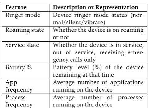
Feature Description or Representation
Ringer mode Device ringer mode status (nor-mal/silent/vibrate)
Roaming state Whether the device is on roaming or not
Service state Whether the device is in service, out of service, receiving emer-gency calls only
Battery % Battery level (%) of the device
remaining at that time App
frequency
Average number of applications running on the device
Process frequency
Average number of processes running on the device
Table 8. Device related features used for call status prediction
a time slot and is computed as
Total # of calls missed Total # of calls received
during the time slot.
• Average call duration - This represents the average call duration for the user during a time slot and is computed as
Total call duration Total # of calls
during the time slot.
• Average call and ring time difference - These represent the average time difference (in minutes) between calls made or calls received by the user during the time slot.
• Average SMS out frequency - This represents the average number of SMS sent by the user (per hour) during the time slot and is computed as
Total # of SMS sent by the user during a time slot
Total # of time slot hours (for that slot) in user’s call history
• Average SMS in frequency - This represents the average number of SMS received by the user (per hour) during the time slot and is computed as
Total # of SMS received by the user during a time slot Total # of time slot hours (for that slot) in user’s call history
Device related features. In addition, the device state at
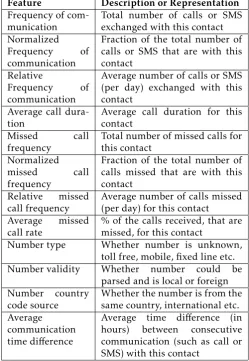
Feature Description or Representation
Frequency of com-munication
Total number of calls or SMS exchanged with this contact Normalized
Frequency of
communication
Fraction of the total number of calls or SMS that are with this contact
Relative
Frequency of
communication
Average number of calls or SMS (per day) exchanged with this contact
Average call dura-tion
Average call duration for this contact
Missed call
frequency
Total number of missed calls for this contact
Normalized
missed call
frequency
Fraction of the total number of calls missed that are with this contact
Relative missed call frequency
Average number of calls missed (per day) for this contact
Average missed
call rate
% of the calls received, that are missed, for this contact
Number type Whether number is unknown,
toll free, mobile, fixed line etc.
Number validity Whether number could be
parsed and is local or foreign
Number country
code source
Whether the number is from the same country, international etc. Average
communication time difference
Average time difference (in
hours) between consecutive
communication (such as call or SMS) with this contact
Table 9. Contact related features used for call prediction
to charge his device before any communication. These factors too can influence a user’s decision to attend calls. Table 8 shows the 6 device related features that we employ. These are:
• Ringer mode - This represents the ringer mode status (normal/silent/vibrate) of the device at the time of call.
• Roaming state - This represents whether the device is on roaming or not at the time of call.
• Service state - This represents the service state of the device i.e. whether it is in service, out of service or receiving emergency calls only at the time of call.
• Battery % - This represents the battery level of the device remaining at the time of call.
• App frequency - This represents the average number of apps running on the device at the time of call.
• Process frequency -This represents the average number of processes running on the device at the time of call.
Caller related features. Moreover, who the the caller is
can also influence a user’s decision to attend a call. If the call is from an important contact, then the user might attend it irrespective of his current situation. Similarly, if a user communicates very frequently with a caller, he/she may be more willing to take the call. On the other hand, if the caller is unknown, then the user may decide to not take the call. Hence, we extract several features for the caller/contact who is calling. Table 9 shows the 12 contact related features we use:
• Frequency of communication - This represents the strength of communication (in the form of total number of calls or SMS exchanged) with this contact.
• Normalized Frequency of communication - This represents the % of the total communication, of the user, that is with this contact (computed as the fraction of the total number of calls or SMS exchanged that are with this contact).
• Relative Frequency of communication - This represents the average number of calls or SMS exchanged per day with this contact and is computed as
Frequency of communication with the contact
Total number of days in user’s communication history
• Average call duration - This represents the average call duration for this contact and is computed as
Total call duration
Total number of calls with this contact
• Missed call frequency - This represents the total number of missed calls for this contact.
• Normalized missed call frequency - This repre-sents the % of calls missed, by the user, that are for this contact and is computed as the fraction of the total number of calls missed.
• Relative missed call frequency - This represents the average number of calls missed per day for this contact and is computed as
Missed call frequency for the contact Total number of days in user’s communication history
Accuracy J48 kNN Naive Bayes Random Forest SMO
0.87 0.77 0.67 0.88 0.83
Table 10. Comparison of accuracies of various classifiers on the DeviceAnalyzer validation set for Call Prediction
and is computed as
Total number of calls missed Total number of calls received
for this contact.
• Number type - This represents the number type i.e. whether it is unknown, toll free, mobile, fixed line etc.
• Number validity - This represents the number validity (whether it could be parsed) and is local or international.
• Number country code source - This represents the country code source i.e. whether the number is from the same country, international etc.
• Average communication time difference - This represents the average time difference (in hours) between consecutive communication (such as a call or SMS) with this contact.
In order to build this model, we extracted these 31 features (13 spatial and temporal, 6 device related and 12 contact related) from the context history of all the users in the DeviceAnalyzer validation set (see Section 3.1). For each user in the validation set, we labeled each instance of an incoming call as either of the 2 classes - ‘Call Taken’ if the call is accepted or ‘Call Missed’ if the call is not accepted by the user. Since the call log data can be unbalanced for many users (with more instances for one class than the other), we applied a resampling filter to introduce a bias towards a uniform class distribution. This filter produces a random subsample of a dataset using either sampling with replacement or without replacement.
We experimented with 5 machine learning tech-niques for this model - J48 Decision Tree, kNN (k=3), Naive Bayes classifier, Random Forest (10 trees) and SMO. These algorithms were run on the validation set with 10 fold cross validation. Table10shows the com-parison of accuracies for these 5 algorithms. Random Forest had the best performance on the data and hence, we have implemented it for Call Acceptance Prediction model.
4.5. Device Charging behavior modeling
Ferreira [11] et al., analyzed the device charging behavior (such as charging time periods, usual battery levels, levels at which charging is initiated, and
Feature Description or Representation
Hashed time
slot
Time of day and Day of week
Semantic Place Semantic Location of the user (Home/Work/Transport etc.)
Mobility state Whether user is moving or
stationary Battery Level
status
Whether battery is very low, low etc.
Charging state Device charging state - con-nected (via ac/usb) or discon-nected
Table 11. Device charging behavior related features
preferred mode of charging) of 4035 participants over a course of 4 weeks. Their study showed that most users follow a pattern in charging their devices. The daily average battery level across all users was 67%. The 2 major charging schedules for most users were between 6 and 8 pm in the evening, when the battery level was at 40%, or between 1 and 2 am in the night when the battery level was at 30%. Also, users preferred to charge their phones via ac for longer periods and usb for shorter periods.
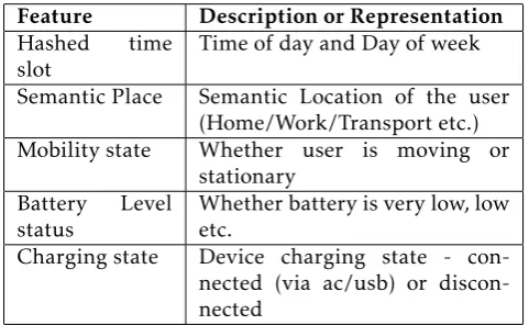
As suggested by this work, we attempted to build such charging behavior models for all users in our DeviceAnalyzer dataset. Table 11 shows the 5 features we employ for modeling users’ device charging behavior. These include:
• Hashed time slot (Time of day and day of week): This feature is important as the time or day can influence a user’s inclination to charge their device. For instance, many users prefer to charge their devices overnight.
• Semantic Place: This represents the semantic location of the user and is generated using the Semantic Place Classification model described in Section 4.3. This feature is intuitive as most people charge their devices at ‘Home’, ‘Work’ or an indoor location.
• Mobility state: This represents whether the user is moving or stationary. People tend to charge their devices in their cars and hence, this feature is important.
extremely low battery levels and there is a significant correlation between the battery level and initiation of charging. Since the device battery level is a numeric value, we discretized it into certain ranges and used the range as a feature. For instance, a battery level of 0 - 20% maps to a range of ‘VeryLow’, from 20 40 % is ‘Low’, from 40 -60% is ‘Average’, from 60 - 80% is ‘High’ and from 80 - 100% is ‘VeryHigh’.
• Charging state: Finally, this represents the device’s charging state - if it is getting charged (via ac/usb) or is disconnected.
These features were used to generate the device charging behavior instances for all the users in the DeviceAnalyzer dataset. To address any imbalance in the dataset, we applied a resampling filter to introduce a bias towards a uniform class distribution. We also filtered out duplicate instances.
To model the charging behavior of users, we employed association rule mining to mine associations between the various features - time period, semantic place, mobility state, battery level and charging status of the device. A significant benefit of association rules is that they can determine strong associations between different attribute values. Thus, they can predict any attribute, not just the class, which gives them the freedom to predict combinations of attributes[29]. We employed two state of the art association rule mining algorithms - Apriori [2] and PredictiveApriori [26]. Apriori iteratively reduces the minimum support until it finds the required number of rules with the given minimum confidence. We set the minimum confidence level as 0.6 and the number of rules to generate as 5. The minimum support is varied from 1.0 to 0.1. PredictiveApriori combines confidence and support into a single measure of predictive accuracy and finds the bestnassociation rules in order. We setnas 5 in our experiments. Some of the sample rules generated for the users in our dataset are:
• If ‘Time slot = Weekday Night’ then ‘Charging State = charging’.
• If ‘Battery Level = Very Low’ and ‘Semantic Place = Home’ then ‘Charging State = charging’.
• If ‘Charging Status=charging’ and ‘Time
slot=Weekend Noon’ then ‘Mobility
State=Stationary’.
• If ‘Time slot = Weekend Night’ and ‘Battery Level=Low’ then ‘Charging State = charging’
Clearly, these rules are intuitive and support the findings in [11]. As evident, users in our dataset charge their phones during weekday or weekend nights, when the battery levels are low and they are at
home. Learning such rules, from a user’s charging behavior, can enable the design of intelligent prompting mechanisms to proactively remind users to charge their devices.
5. Evaluation
5.1. Methodology and Goals
As stated earlier, the Learning Engine of the Rover II middleware is responsible for building diverse user behavioral models in order to predict a user’s behavior and enable the middleware to take proactive actions on the user’s behalf. Hence, the primary goal of our evaluation is to determine how accurately the various algorithms and approaches, that we have implemented as part of the engine, model users’ behavior. To this end, we evaluate the approaches that we have implemented currently (for Mobility State Classification, Semantic Place Classification and Call Acceptance Prediction) on the entire dataset of 200 users from the DeviceAnalyzer data collection as well as the dataset collected from the field study (see Section3) with 10 fold cross validation. We perform an accuracy analysis of these approaches and report our results.
5.2. Accuracy measures used
Since these models involve binary and multi-label classification, we define accuracy for them as:
a = T∩P T∪P
where T is the set of ground truth and P is the set of predicted labels for all instances.
5.3. Results
Table15 shows the overall accuracy results for all the approaches that have been implemented as part of the Learning Engine in Rover II. As evident, they achieve high accuracy. We now discuss the accuracies of the individual models that have been implemented.
Semantic Place Classification. Table12 shows the
Semantic Place Label
Accuracy Home Work InRec OutRec Transport InKnown OutKnown NearHome NearWork Other
1.0 0.95 0.93 0.78 0.81 0.94 0.9 0.96 0.95 0.76
Table 12. Individual place accuracies for Semantic Place Classification
Ground Truth Predicted labels Stationary Moving
Stationary 0.85 0.15
Moving 0.07 0.93
Table 13. Confusion matrix for Mobility State Classification
Ground Truth Predicted labels
Call Taken Call Missed
Call Taken 0.91 0.09
Call Missed 0.13 0.87
Table 14. Confusion matrix for Call Acceptance Prediction
Model Accuracy (%)
Semantic Place Classification 89.8 Mobility State Classification 88.02
Call Acceptance Prediction 89.1
Table 15. Accuracy of various algorithms (%)
we observed that the correct labels for some of these places were interchanged. Overall, our algorithm has an accuracy of 89.8 %.
Mobility State Classification. Table13shows the
confu-sion matrix for Mobility State Classification. Overall, this approach has an accuracy of 88.02% and can accu-rately classify the user’s mobility state.
Call Acceptance Prediction. Table14shows the confusion
matrix for Call Acceptance Prediction. Our approach achieves an accuracy of 89.1% and can accurately determine whether a user would accept an incoming call.
6. Related Work
Since our work involves building several user behavior models for semantic place classification, mobility state classification, call acceptance prediction etc. we have categorized the related work into different sections. We differentiate our work from them and identify their shortcomings. Please note that while most of these works have focused on building a single isolated user model, we have developed a unified infrastructure for building several such models, from large-scale smartphone data, as part of the generic Rover II context-aware middleware.
6.1. Semantic Place Classification
Previous research in Semantic Place Classification has used the MDC dataset [16,18] for classifying semantic places into 10 categories specified by the challenge organizers (Home, Home of a friend, Work, Transport, Indoor sports, Outdoor sports etc.). Huang et al. [13] used 54 features and experimented with classifiers such as kNN, Support Vector Machines (SVM) and J48 along with an ensemble of the three to achieve a final accuracy of 65.77% with 10 fold cross validation. Montoliu et al. [22] employed a multi-coded class based multiclass evaluation rule that combines classification results of the binary classifiers such as kNN and SVM. They achieve an accuracy of 73.26% with 2 fold cross validation. Zhu et al. [31] compare the performance of Logistic Regression, SVM, Gradient Boosted Trees (GBT), and Random Forest to achieve an accuracy of 65.3% with GBT and 10 fold cross validation. Lex et al. [19] used 32 features and employed Random Forest as well as SVM. They achieve an accuracy of 85.4% with RandomForest and 10-fold cross-validation. While some of the features employed by these works overlap with ours, a direct comparison with them is not possible due to difference in the datasets, quality of location information, and semantic place labels. However, the overall accuracy of our Semantic Place Classification algorithm is higher.
More recently, Bao et al. [4] have experimented with the DeviceAnalyzer dataset and employed features such as Wi-Fi visibility and connectivity, and cell locations to identify semantic places such as Home, Work and Commute as well as the transitions between them. However, they do not present any evaluation or results.
6.2. Mobility State
While previous work in activity recognition (including SenseMe [5], CenceMe [21] and Jigsaw [20]) has focused on fine-grained activity recognition such as Walking, Running, Driving etc. , it is not possible to do that with the DeviceAnalyzer dataset because of the limited accelerometer data available and its sampling rate (see Section 4.1). Hence, due to this inherent limitation of the used dataset, our work focuses on determining two mobility states for the user - Moving and Stationary.
6.3. Call Acceptance Prediction
availability for phone calls. They used 3 basic features such as time of the day, day of the week and location, and predicted the user’s availability and likelihood of accepting phone calls based on a weighted average of these feature values. They evaluated their approach on the data of 10 users from the Reality Mining dataset [7] and appear to have achieved an average accuracy of around 50%. This makes their approach highly unsuitable for real world applications. While our approach shares similar goals with these works, we use 31 varying contextual features for call acceptance prediction. In comparison to these works, our approach has a much higher accuracy (89%) for 200 users.
6.4. Device charging behavior
Existing literature [15,23,25] has explored correlations between device power consumption and a user’s context (such as location, time and device usage) as well as device related features (such as CPU utilization, wireless state, IO and data transfer) in order to perform context-aware and personalized device battery lifetime and level prediction. However, majority of this research is driven by the need for effective energy management on devices. To the best of our knowledge, no other work has proposed modeling a user’s charging behavior to generate patterns and rules in order to design intelligent prompting or reminder mechanisms.
6.5. User modeling from mobile phone data
The Reality Mining project [7] was one of the first attempts at mobile phone data collection. This project collected data from 100 users over the course of 9 months. However, a large amount of data collected in this study was through self reported surveys. Eagle and Pentland [8] applied principal component analysis to users’ location data from this dataset to identify primary routines or eigenbehaviors (such as sleeping late on weekends or going out on weekend nights) for individuals and their social circle. They also inferred community affiliations by clustering individuals. Altshuler et al. [3] used the same dataset for predicting individual traits of users such as their nationality, gender and social links such as life partners. Farrahi [10] explored the use of topic modeling for discovering location driven routines such as ‘going to work’ or ‘staying home at evening’ and experimented with this approach on a subset of the Reality Mining dataset. In contrast, we attempt to build diverse behavioral models that capture different aspects of users’ behavior (such as place visitation patterns, calling patterns and device charging behavior) from large-scale data collected over several years.
Srinivasan et al. [27] proposed an association rule mining based algorithm to mine co-occurring context patterns of users on their devices. A limitation of
their work is that though they determine correlations between inferred contexts of users such as ‘AtHome’ and ‘ReadComics’, they do not explain how the inference is performed. Moreover, their approach is restricted to pattern mining only and cannot predict or classify user behavior which is often more important and accurate. On the other hand, we employ several machine learning techniques including classifiers and association rules to build user behavioral models.
7. Conclusion and future work
In this paper, we explored learning diverse patterns from large-scale data collected from users’ smart-phones. We utilized these patterns to help identify a variety of the users’ behaviors, habits, and daily life places and activities. To this end, we developed a unified infrastructure and implemented several novel approaches and algorithms that employ various contex-tual features and state of the art machine learning tech-niques for building behavioral models of users. Exam-ples of generated models include classifying users’ semantic places and mobility states, predicting their availability for accepting calls and modeling their device charging behavior. We evaluated our work on large-scale real-world smartphone data of 200 users, from the DeviceAnalyzer dataset, consisting of 365 million data points. We showed that our algorithms and approaches can model user behavior with high accuracy and demonstrate improved performance over existing work.
We are currently working on building several other models such as predicting the next called contact for a user, as well as battery lifetime for his device. In future, we plan to work on more advanced models such as predicting users’ sleep cycles, classifying their personalities in terms of the Big Five personality model, and inferring their moods based on their smart phone usage. We also plan to investigate community models which utilize the power of crowd sourcing and group behavior. In addition, we are working on analyzing
behavioral sequences which are behaviors that follow each other (for instance, charging phone after reaching home, sending an SMS after missing a call etc.) and modeling them using HMMs. Our ultimate goal is to enable Rover II to act as an intelligent personal digital assistant and take proactive actions on the users’ behalf.
References
[1] E. Achtert, H.-P. Kriegel, and A. Zimek. Elki: a software system for evaluation of subspace clustering algorithms. InScientific and Statistical Database Management, pages 580–585. Springer, 2008.
[3] Y. Altshuler, N. Aharony, M. Fire, Y. Elovici, and A. Pentland. Incremental learning with accuracy prediction of social and individual properties from mobile-phone data. In 2012 International Conference on Privacy, Security, Risk and Trust (PASSAT) and 2012 International Confernece on Social Computing (SocialCom). IEEE, 2012.
[4] X. Bao, Y. Shen, N. Z. Gong, H. Jin, and B. Hu. Connect the dots by understanding user status and transitions. In
Adjunct Proceedings of the 2014 ACM International Joint Conference on Pervasive and Ubiquitous Computing. [5] P. Bhargava, N. Gramsky, and A. Agrawala. Senseme:
a system for continuous, on-device, and multi-dimensional context and activity recognition. In
Proceedings of the 11th International Conference on Mobile and Ubiquitous Systems: Computing, Networking and Services, 2014.
[6] P. Bhargava, S. Krishnamoorthy, and A. Agrawala. An ontological context model for representing a situation and the design of an intelligent context-aware middleware. In Proceedings of the ACM Conference on Ubiquitous Computing, 2012.
[7] N. Eagle and A. Pentland. Reality mining: sensing complex social systems. Personal and ubiquitous computing, 10(4):255–268, 2006.
[8] N. Eagle and A. S. Pentland. Eigenbehaviors: Identifying structure in routine.Behavioral Ecology and Sociobiology, 63(7):1057–1066, 2009.
[9] M. Ester, H.-P. Kriegel, J. Sander, and X. Xu. A density-based algorithm for discovering clusters in large spatial databases with noise. InKdd, volume 96, pages 226–231, 1996.
[10] K. Farrahi and D. Gatica-Perez. What did you do today?: discovering daily routines from large-scale mobile data. InProceedings of the 16th ACM international conference on Multimedia, 2008.
[11] D. Ferreira, A. K. Dey, and V. Kostakos. Understanding human-smartphone concerns: a study of battery life. In
Pervasive computing, pages 19–33. Springer, 2011. [12] M. Hall, E. Frank, G. Holmes, B. Pfahringer, P.
Reute-mann, and I. H. Witten. The weka data mining software: An update. SIGKDD Explor. Newsl., 11(1):10–18, Nov. 2009.
[13] C.-M. Huang, J. J.-C. Ying, and V. S. Tseng. Mining users’ behaviors and environments for semantic place prediction. In Nokia Mobile Data Challenge 2012 Workshop. p. Dedicated task, volume 1, 2012.
[14] H. Husna, S. Phithakkitnukoon, E.-A. Baatarjav, and R. Dantu. Quantifying presence using calling patterns. In3rd International Conference on Communication Systems Software and Middleware and Workshops,. IEEE, 2008. [15] Y. Jiang, A. Jaiantilal, X. Pan, M. A. Al-Mutawa,
S. Mishra, and L. Shi. Personalized energy consumption modeling on smartphones. In Mobile Computing, Applications, and Services, pages 343–354. Springer, 2013. [16] N. Kiukkonen, J. Blom, O. Dousse, D. Gatica-Perez, and J. Laurila. Towards rich mobile phone datasets: Lausanne data collection campaign.Proc. ICPS, Berlin, 2010. [17] S. Krishnamoorthy, P. Bhargava, M. Mah, and
A. Agrawala. Representing and managing the context
of a situation. The Computer Journal, 55(8):1005–1019, 2012.
[18] J. K. Laurila, D. Gatica-Perez, I. Aad, O. Bornet, T.-M.-T. Do, O. Dousse, J. Eberle, M. Miettinen, et al. The mobile data challenge: Big data for mobile computing research. InPervasive Computing, number EPFL-CONF-192489, 2012.
[19] E. Lex, O. Pimas, J. Simon, and V. Pammer-Schindler. Where am i? using mobile sensor data to predict a userŠs semantic place with a random forest algorithm. In
Mobile and Ubiquitous Systems: Computing, Networking, and Services, pages 64–75. Springer, 2013.
[20] H. Lu, J. Yang, Z. Liu, N. D. Lane, T. Choudhury, and A. T. Campbell. The jigsaw continuous sensing engine for mobile phone applications. InProceedings of the 8th
ACM Conference on Embedded Networked Sensor Systems,
2010.
[21] E. Miluzzo, N. D. Lane, K. Fodor, R. Peterson, H. Lu, M. Musolesi, S. B. Eisenman, X. Zheng, and A. T. Campbell. Sensing meets mobile social networks: the design, implementation and evaluation of the cenceme application. InProceedings of the 6th ACM conference on Embedded network sensor systems, 2008.
[22] R. Montoliu, A. Martínez-Uso, J. Martínez-Sotoca, and J. McInerney. Semantic place prediction by combining smart binary classifiers. InNokia Mobile Data Challenge 2012 Workshop. p. Dedicated task, volume 1, 2012. [23] E. Oliver and S. Keshav. Data driven smartphone energy
level prediction. University of Waterloo Technical Report, 2010.
[24] J. Platt et al. Fast training of support vector machines using sequential minimal optimization. Advances in kernel methods-support vector learning, 3, 1999.
[25] N. Ravi, J. Scott, L. Han, and L. Iftode. Context-aware battery management for mobile phones. InSixth Annual IEEE International Conference on Pervasive Computing and
Communications, 2008.
[26] T. Scheffer. Finding association rules that trade support optimally against confidence. In Principles of
Data Mining and Knowledge Discovery, pages 424–435.
Springer, 2001.
[27] V. Srinivasan, S. Moghaddam, A. Mukherji, K. K. Rachuri, C. Xu, and E. M. Tapia. Mobileminer: Mining your frequent patterns on your phone. InProceedings of the 2014 ACM International Joint Conference on Pervasive and Ubiquitous Computing.
[28] D. Wagner, A. Rice, and A. Beresford. Device analyzer: Understanding smartphone usage. In10th International Conference on Mobile and Ubiquitous Systems: Computing, Networking and Services, Tokyo, Japan. 2013.
[29] I. H. Witten and E. Frank.Data Mining: Practical machine learning tools and techniques. Morgan Kaufmann, 2005. [30] H. Zhang and R. Dantu. Quantifying the presence of
phone users. In5th IEEE Consumer Communications and Networking Conference, 2008.