A Gaussian mixture method for specific differential phase retrieval
at X-band frequency
Guang Wen, Neil I. Fox, and Patrick S. Market
School of Natural Resources, University of Missouri, 332 ABNR Building, Columbia, Missouri 65201, USA Correspondence:Neil I. Fox ([email protected])
Received: 8 May 2019 – Discussion started: 13 May 2019
Revised: 27 August 2019 – Accepted: 21 September 2019 – Published: 23 October 2019
Abstract. The specific differential phaseKdp is one of the
most important polarimetric radar variables, but the variance σ2(Kdp), regarding the errors in the calculation of the range
derivative of the differential phase shift8dp, is not well
char-acterized due to the lack of a data generation model. This paper presents a probabilistic method based on the Gaus-sian mixture model forKdpestimation at X-band frequency.
The Gaussian mixture method can not only estimate the ex-pected values ofKdpby differentiating the expected values of
8dp, but also obtainσ2(Kdp)from the product of the square
of the first derivative of Kdp and the variance of 8dp.
Ad-ditionally, the ambiguous phase and backscattering differ-ential phase shift are corrected via the mixture model. The method is qualitatively evaluated with a convective event of a bow echo observed by the X-band dual-polarization radar in the University of Missouri. It is concluded that Kdp
es-timates are highly consistent with the gradients of 8dp in
the leading edge of the bow echo, and largeσ2(Kdp)occurs
with high variation ofKdp. Furthermore, the performance is
quantitatively assessed by 2-year radar–gauge data, and the results are compared to linear regression model. It is clear that Kdp-based rain amounts have good agreement with the
rain gauge data, while the Gaussian mixture method gives improvements over the linear regression model, particularly for far ranges.
1 Introduction
Apart from radar reflectivity (ZH) and differential
reflec-tivity (ZDR), polarimetric radars also obtain the differential
phase shift (8dp) to reflect the forward-scattering property
of hydrometeor scatterers (Seliga and Bringi, 1978;
Sachi-dananda and Zrni´c, 1986). Its range derivative, also called the specific differential phase (Kdp), has some advantages
overZH andZDR(Zrni´c and Ryzhkov, 1996), including
in-sensitivity to attenuation, clutter, partial beam blockage, and radar absolute calibration. The specific differential phase has played a key role in various meteorological applications – such as hydrometeor classification (Lim et al., 2005; Park et al., 2009), raindrop size distribution retrieval (Bringi et al., 2002; Williams et al., 2014), and quantitative precipitation estimation (Ryzhkov et al., 2005; Cifelli et al., 2011) – since Kdp is a phase variable independent ofZH andZDRand
al-most linearly proportional to rain rate.
A linear regression model has been developed to derive Kdp from the slope of the range profile of 8dp measured
by the polarimetric radars. In Hubbert et al. (1993),8dp is
first processed by a light filter that attenuates the8dp
magni-tudes within a scale of 375 m by 10 dB, and it is then heav-ily smoothed in 1.5 km by 10 dB. An iterative filtering tech-nique is used for eliminating nonzero backscattering differ-ential phase shift (Hubbert and Bringi, 1995). The filtered 8dpmeasurements are finally fitted into a first-order
polyno-mial to estimate the8dp slope in a given window. Liu et al.
(1993) supply the accuracy of meanKdpas±0.25◦km−1
us-ing 128 pulses, while Aydin et al. (1995) indicate that the accuracy is within±0.5◦km−1for a heavy rainfall event us-ing 64 pulses. On the other hand, Ryzhkov and Zrni´c (1996) produce two kinds ofKdpfor S-band radars: one is obtained
over 16 range gates (2.4 km) forZH ≤40 dBZ, and the other
is produced over 48 gates (7.2 km) forZH>40 dBZ.
Nega-tiveKdpis incorporated into the rain rate algorithm to avoid
bias in the low rain rate. The analyses of 15 storms show that the standard error ofKdpis 0.04–0.10◦km−1for heavily
either 128 or 64 pulses. Vulpiani et al. (2012) develop a mul-tistep moving-window approach based on the linear regres-sion model to handle the8dp folding and other ambiguous
data. This approach is applicable to the complex terrain but still valid for various topographical environments.
X-band dual-polarization radars have drawn increasing at-tention in the radar meteorology community in recent years on account of their low cost, fine resolution, and high sensi-tivity to light precipitation (Chandrasekar et al., 2012; Lim et al., 2013; Berne and Krajewski, 2013; Kalogiros et al., 2014; Oue et al., 2016). In the literature, X-band algorithms have been proposed forKdpestimation. For example, the
lin-ear regression method is adapted for the X-band radar data and used to retrieve rainfall (Matrosov et al., 2006). The am-biguous8dpis naturally corrected by examining the complex
values of the range profiles of 8dp exponentials, and Kdp
is then estimated by a regularization framework based on a cubic spline smoothing (Wang and Chandrasekar, 2009). In this method, the bias and variance are adjustable through the smoothing parameter, giving high spatial resolutions ofKdp
estimates. Moreover, algorithms of linear programming (Gi-angrande et al., 2013) and Kalman filter (Schneebeli et al., 2014) have also been applied to the Kdp estimation,
yield-ing good performance for rainfalls and snowfalls. It is no-ticeable that the Kalman filter method minimizes the Gaus-sian error function to obtain the mean profile ofKdp. It gives
a significant improvement on the Kdp mean, particularly in
the small-scale structure with high peaks. In addition, the 8dp measurements at X-band frequency are affected by the
backscattering differential phase shiftδco. The constraints of
Kdp−ZH−ZDRandδco−ZDRcan be used to improve the
estimation of Kdp and δco (Otto and Russchenberg, 2011;
Reinoso-Rondinel et al., 2018), although these constraints are only valid in the rain regime.
The recent algorithms are focused on the improvement of estimating the meanKdp, whereas its variance σ2(Kdp)is
not well characterized due to the lack of a data generation model. TheKdpvariance is often inherited from the8dp
vari-ance σ2(8dp)
, leading to large relative errors for lowKdp
with a fixed path length. As noted by Gorgucci et al. (1999), theKdpestimated by the linear regression has large errors in
the nonuniform rain media, while the errors increase when the radar reflectivity presents large gradients in dimensions. In this study, we propose a probabilistic method based on the Gaussian mixture model for Kdp estimation at X-band
fre-quency. The Gaussian mixture method can not only estimate the expected values ofKdpby differentiating the conditional
expectation of8dp, but also yieldσ2(Kdp)by regarding the
errors in the calculation of the first derivative of 8dp. It is
found thatσ2(Kdp)is closely related to the square of the first
derivative ofKdpandσ2(8dp), while a largeσ2(Kdp)is
asso-ciated with high variation ofKdpestimates. When compared
to the existing methods, our method considers the joint prob-ability density function of the data as the nonlinear Gaussian mixture, leading to better performance for the multimodal
data. Since theKdp variance is nonconstant, it leads to the
variability in theKdp error characteristics. We can then use
theKdp variance to calculate the variances ofZH andZDR
via the attenuation correction, as well as the variance of rain rate via theR–Kdp relation. These variances are useful for
studying the propagation of uncertainty in the weather model and the streamflow trends in the hydrological model.
The paper is organized as follows. Section 2 provides background information aboutKdpand the Gaussian mixture
model. Section 3 describes the radar and gauge data. Sec-tion 4 presents the methodology. We first remove the residual clutter using data masks (Sect. 4.1) and then derive the joint probability density function to estimate the expected value of 8dpandσ2(8dp)(Sect. 4.2). Next, we correct the ambiguous
phase andδcovia the mixture model (Sect. 4.3). Last, we
cal-culate the expected value and variance ofKdp(Sect. 4.4) and
improve theKdpprofile by reducingσ2(Kdp)(Sect. 4.5). To
evaluate the algorithm, Sect. 5 gives a case study and a com-parison between the radar and gauge. Section 6 summarizes the paper.
2 Background
The specific differential phase is the first derivative of the differential phase shift8dp along the radar range, giving a
way to estimateKdpby radar measurement of8dp.
Further-more, the probability density function of8dp can be
mod-eled as a Gaussian mixture, which is often obtained via an expectation–maximization (EM) approach. The mean and variance of the Gaussian mixture may lead to the improve-ment of theKdpestimation.
In this section, we introduce the physical interpretation of Kdp and the regression model for estimatingKdp. Since the
Gaussian mixture is adopted as the data generation model, we also give a brief description of the mathematical definition of the Gaussian mixture model and the EM approach.
2.1 Specific differential phase (Kdp)
For linear polarization,Kdpis proportional to the integral of
the raindrop size distribution and the real part of the differ-ence of forward-scattering amplitudes at orthogonal polar-izations. It is mathematically formulated as
Kdp=
0.18λ π
∞ Z
0
N (D)· <fhh(0, D)−fvv(0, D)
dD
(◦km−1), (1)
whereλ is radar wavelength in millimeters, D is raindrop size in millimeters, N (D) is size spectrum in cubic me-ters per millimeter (m3mm−1), andfhh,vv(0, D)is
1/λ2, leading to the fact thatKdpis inversely proportional to
radar wavelength, i.e., Kdp∝1/λ. Therefore, the values of
Kdpat the X band are often larger than that at the S band by
a factor of 3, indicating that X-band radar can provide better Kdpdata than S-band radar when retrieving the rainfall rate.
The conclusion is still valid even if the Mie effect is taken into account (Bringi and Chandrasekar, 2001; Chandrasekar et al., 2006).
However,Kdpcannot be detected by polarimetric radar
di-rectly, whereas its integral 8dp is measurable. Hence,Kdp
can be estimated as the range derivative of the profile of8dp,
i.e.,Kdp= 18dp
21r , whereris the radar range in kilometers. An
alternative approach to estimatingKdp is to apply a
regres-sion fit to the profile of8dp, and the first-order polynomial is
usually considered as the fitting function (Balakrishnan and Zrni´c, 1990; Ryzhkov and Zrni´c, 1995). Subsequently, if the 8dp measurements are equally spaced in range by1r,Kdp
is then estimated by Kdp=
Pn
i=18dp(ri)[6i−3(n+1)1r]
n(n−1)(n+1)1r2 , (2)
wherenis the number of gates. Equation (2) shows that the accuracy of Kdp estimates is determined by the number of
gates (n) and the accuracy of 8dp. By assumingσ2(8dp)
is relatively stable for all gates along a ray and noting that 8dp(ri)is the only variable in Eq. (2),σ2(Kdp)is formulated
as
σ2 Kdp=
3σ2 8dp
1r2[n(n−1)(n+1)]. (3)
In Eq. (3), σ2 Kdp is proportional to σ2 8dp, which is
related to the spectrum width, cross-correlation coefficient, and the dwell time (Sachidananda and Zrni´c, 1986; Hubbert et al., 1993), and inversely proportional to n3. This method has been widely used in the existing radar system (Cifelli et al., 2018; Chandrasekar et al., 2018; Chen et al., 2017b, c). The details of the regression-based estimation ofKdpare
given in Bringi and Chandrasekar (2001) and Appendix A. Moreover, it is notable that the backscattering phase shift is not negligible at the X band; thus the total propagation phase shift(9dp)consists of8dpand the backscattering
dif-ferential phase,δco; i.e.,9dp=8dp+δco. The
backscatter-ing phase shift is often shown as a sudden jump over one or a few range gates in a monotonically increasing9dp profile
of rain (May et al., 1999), with a value much larger than the standard deviationσ 9dp. The presence ofδcoover a small
number of consecutive gates can be eliminated by a simple filter (Hubbert and Bringi, 1995).
The specific differential phase is a unique polarimetric variable in terms of statistical errors in the rain rate estima-tion, since it is the range derivative of the phase measurement
2.2 Gaussian mixture model
The Gaussian mixture is a statistical model for data proba-bility density estimation, assuming that the data points are generated by a mixture of a finite number of Gaussian distri-butions associated with their weights (McLachlan and Peel, 2000; Sung, 2004). Intuitively, it is used to model the multi-modal data, with each Gaussian component corresponding to a subpopulation of the data. The mathematical formulation is given as
f (z)=
m X
i=1
wiN z;µi,6i, (4)
where m is the number of components in the Gaus-sian mixture, wi is a weight with Pmi=1wi =1, and
N z;µi,6i
is the ith Gaussian distribution with mean µi and covariance 6i; i.e., N z;µi,6i
=
(2π )k6i
−1/2
exph−1
2(z−µi)T6−1i (z−µi) i
, where
kis the data dimension.
It is prevalent to use an Expectation–Maximization (EM) algorithm to estimate the parameters,w,µ, and6, by con-structing the lower bound of the log-likelihood based on Jensen’s inequality (Dempster et al., 1977). The EM algo-rithm is divided into two steps, namely, an expectation (E) step and a maximization (M) step. In the E step, a degree of membership toward to thejth cluster is calculated; i.e., Qij =p
y(i)=j|x(i);w,µ,6, (5) whereiis theith data with a total number ofndata points, and y is a latent variable that determines the correspond-ing cluster. Here,Qgives a tight lower bound for the log-likelihood, equivalent to maximizing the expectation. In the M step, the exact form of the lower bound based on Jensen’s inequality is expressed as
L(w,µ,6)=X
i X
j
Qij
log
exph−1
2(xi−µ)T6
−1(xi−µ)iw j
q (2π )k6
Qij
. (6)
By maximizing the lower bound with respect to each param-eter,wj,µj, and6j are updated as (Petersen and Pedersen,
wj = P
iQij
n , (7)
µj = P
iQijx(i) P
iQij
,and (8)
6j = P
iQij(x(i)−µj)(x(i)−µj)T P
iQij
,respectively. (9)
Notably, the M step increases the log-likelihood monotoni-cally, if the covariance6j is a positive-definite matrix. Fi-nally, the E step and M step are iteratively operated until the log-likelihood converges to a value with the difference between two successive steps below a certain threshold. In addition, the EM algorithm requires a specification of the number of clusters, m, prior to the E and M steps, and an inappropriate choice ofmmay lead to meaningless values of the parameters. To tackle this problem, the Bayesian infor-mation criterion is often calculated to select the optimalm, while a Dirichlet process may also be used to model a prior probability to construct an infinite Gaussian mixture.
One of interpretations of the Gaussian mixture is to view each distribution as a cluster with a Gaussian probability den-sity, while the individual data point is attributed to a spe-cific cluster or a weight toward the cluster, regarded as unsu-pervised learning (Hastie et al., 2009). The clustering pro-cedures based on the Gaussian mixture model have been applied to the identification of storm structure (Veneziano and Villani, 1996), as well as the particle identification at S-band (Wen et al., 2015, 2016b, 2017) and X-band (Wen et al., 2016a) frequencies. Furthermore, the Gaussian mix-ture model can be extended to fit a set of unknown parameters in the prior probability of the Bayesian framework, forming a Bayesian–Gaussian mixture model (Li et al., 2012). The prior is then multiplied with the known conditional proba-bility of data given the parameters to be estimated, yielding the posterior probability with a new set of parameters. The expectation of the posterior is often used to retrieve the con-ditional mean of the new parameters based on least squares criteria.
For the regression problem, the characteristics of the Gaus-sian mixture imply that the direct modeling of a regression function is very difficult. Nevertheless, the joint probability of the measurements and the estimated parameters may be modeled as a Gaussian mixture, leading to a regression func-tion derived from the joint density model. Due to the asymp-totic consistency of a Gaussian mixture model, it is capable of estimating a general density function inRn in any shape (Sung, 2004). Moreover, the speed of calculating unknown parameters within a Gaussian mixture linearly depends on the number of the training data points, and the computation of the outputs is independent of the size of the training data. Consequently, regression based on a Gaussian mixture can be achieved very rapidly, compared to Gaussian process
re-gression that grows with the data size. In addition, the Gaus-sian mixture can also be used to solve the regression problem with multiple dimensions, and a subset of dimensions can be selected to handle the missing data (Wen et al., 2015).
3 Data
As part of the Missouri Experimental Project to Stim-ulate Competitive Research (EPSCoR), an X-band dual-polarization radar in the University of Missouri (MZZU) was deployed at the South Farm Research Center (38.906◦N, 92.269◦W) in the Midwest of America in the summer of 2015. The details of the radar characteristics are described in Simpson and Fox (2017). The primary objective is to provide the observations of precipitation near the surface by means of low-cost and fine-scale X-band radar and to fill the ob-servational gaps of the S-band radar network in Saint Louis (KLSX), Kansas City (KEAX), and Springfield (KSGF). Within the MZZU radar coverage, the Hinkson Creek located near Columbia, MO, flows through a catchment basin and eventually merges into the Missouri River, forming a typi-cal urban watershed (Hubbart and Zell, 2013). The radar can provide timely flash flooding warning for the Hinkson Creek watershed and surrounding areas.
In this study, we analyze the data collected by the X-band MZZU dual-polarization radar. The maximum unam-biguous range of the MZZU radar is 94.64 km with a reso-lution of 260 m in range and 1◦ in azimuth. During the ob-servational periods, the radar operates in a volumetric scan-ning mode of nine elevations at 0.8, 2, 3, 4, 5, 6, 7, 8.5, and 10◦, updated every 4 min. The raw radar data are
or-ganized and processed by an open-source software package called the Python ARM Radar Toolkit (Py-ART: Helmus and Collis, 2016). Moreover, to validate theKdpestimation
algo-rithm, we also use the data from tipping-bucket rain gauges in the Missouri Mesonet weather station network, includ-ing Bradford Farm (38.897◦N, 92.218◦W), Sanborn Field (38.942◦N, 92.320◦W), Auxvasse (39.089◦N, 91.999◦W), and Williamsburg (38.907◦N, 91.734◦W). The horizontal distances between the rain gauges and the radar center are 4.4, 6.0, 30.8, and 46.2 km, respectively. The first elevations at Bradford and Sanborn may be affected by ground clut-ter, since the radar beams are very close to the ground, with heights of 314.6 and 336.9 m a.s.l., respectively, including the radar tower. Therefore, the second elevation at 2◦is se-lected for validation. In contrast, the first elevations at Aux-vasse and Williamsburg reach about 723.8 and 999.0 m a.s.l., which are less contaminated by ground clutter. Furthermore, the point measurement of the rain gauge is different from the volumetric measurement of radar, imposing additional errors on the comparison between the radar and gauge (Anagnos-tou et al., 1999). The radar-based rain rate is then derived by averagingKdpover three successive range gates and three
rainfall time.
Sites Mean SD Max Total Duration (mm) (mm) (mm) (mm) (h)
Bradford 2.1 3.5 38.1 2224.9 1080 Sanborn 2.0 3.3 43.7 2181.4 1082 Auxvasse 2.0 3.3 38.4 2284.3 1144 Williamsburg 2.1 3.7 40.1 2495.9 1191
over each gate in order to obtain good consistency between the instruments. In addition, the rain gauges are carefully calibrated in terms of instrumentation failure, clogging, and other discrepancies between the devices (Simpson and Fox, 2017) and are well documented to provide long-term data for rainfall observations.
Table 1 summarizes the characteristics of rainfalls ob-served at Bradford, Sanborn, Auxvasse, and Williamsburg between April 2016 and June 2018. It is clear that the hourly rain amounts are dominated by light rain, with similar means of 2.0–2.1 mm at the four sites, indicating uniformly dis-tributed rainfalls within the experimental region. On the other hand, the standard deviations of Bradford and Williamsburg are 3.5 and 3.7 mm, respectively, a little larger than that of 3.3 mm at Sanborn and Auxvasse. Moreover, Sanborn gives the highest hourly rain amount, the lowest total rain amount, and the second lowest duration out of the four sites, due to the effects of the urban heat island (Hubbart et al., 2014). The second highest maximum hourly rain amount is recorded at Williamsburg; however, the total rain amount and duration are also the highest among the four sites, implying that con-vective rain is the most frequent at Williamsburg. In contrast, stratiform rain is more common at Bradford, since the gauge records the lowest maximum hourly rain amount and dura-tion, as well as the second total hourly rain amount. In addi-tion, it can be seen that Auxvasse also provides useful data for the comparisons between gauges and between the radar and gauge, though the statistics are all ranked in the middle of the four sites. Overall, the rain gauge data at Bradford, Sanborn, Auxvasse, and Williamsburg are representative and sufficiently large, leading to a valid dataset for testing the KdpandKdp-based rain amounts.
4 Kdpretrieval
As discussed in Sect. 2, the joint probability density function (PDF) based on a Gaussian mixture can be used to derive the regression model forKdpestimation. The Gaussian
mix-ture method (GMM) not only estimates the expected values ofKdpby differentiating the conditional expectation of8dp,
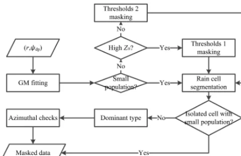
Figure 1. Flowcharts of Kdp estimation algorithms used in the MZZU radar:(a)linear regression model and(b)Gaussian mixture method.
but also gives an estimation of Kdp variance by regarding
the errors in the calculation of the first derivative of8dp. In
this section, we describe GMM for theKdpestimation using
MZZU radar data. Figure 1 illustrates the flowchart of GMM (Fig. 1b), comparing to that of the linear regression model (LR; Fig. 1a).
From the chart of LR in Fig. 1a, we can see that after the radar measurements are collected, the9dp is unfolded and
then the clutter is removed. After these corrections, an itera-tive filtering method is applied to the9dpprofile. An adaptive
method is finally used to estimate theKdp profile according
to the values of ZH. The Gaussian mixture model, on the
other hand, processes9dpdifferently. First of all, the clutter
is masked out according to the thresholds ofZHand the
vari-ation of9dp. Secondly, the rangerand9dpare fitted into a
Gaussian mixture to yield the joint PDF, while the9dpmean
and the9dpvariance are obtained by taking the first raw and
second central moments of the conditional PDF of9dpgiven
r. Thirdly, some specific clusters in the Gaussian mixture PDF are adjusted to solve the problems of ambiguous9dp
and backscattering differential phase shiftδcoin order to
de-rive the PDF of8dp. Fourthly, a rawKdpprofile is calculated
from the first derivative of the expected values of8dp, and
the associated variances are obtained via a Taylor series ex-pansion. Finally, the rawKdpprofile is smoothed, and,
conse-quently, the variances are reduced. In addition, new8dpwith
Figure 2.Flowchart of data masking.
4.1 Data masking
The presence of clutter in the 9dp measurements may
severely affect the Kdp estimation, producing significantly
large variations on the estimates. It is well known that the effect of clutter can be reduced by applying a spectrum filter to the time-series data (e.g., May and Strauch, 1998; Hub-bert et al., 2009). However, some residual clutter echoes are still shown on the radar measurements including9dp (Wen
et al., 2017). Therefore, the clutter needs to be well handled in GMM, prior to the deviation of the regression model based on the joint PDF.
In LR, the clutter is often eliminated by some criteria based on 9dp or ρhv. For instance, we use the thresholds
of the local standard deviation of9dpless than 10◦to
clas-sify valid points. Further, 10 consecutive range gates of valid points signify the beginning of a rain cell, and 5 consecutive gates of invalid points finish the associated rain cell. Overall, the thresholds give a fairly good performance on the MZZU radar; however, the clutter may be incorrectly identified in the regions of high reflectivity or for the echoes mixed by weather and clutter, which are often associated with large 9dpvariation.
In contrast, GMM adopts sophisticated procedures, as de-picted in Fig. 2. It is clear that there are five stages in the data masking, beginning with the input of raw 9dp and ending
with masked data. At the first stage, the raw data are fitted to a Gaussian mixture initialized by thek-means clustering, while the covariance is set to be diagonal for simplicity. The clusters with no more than five points are promptly masked out, before they pass to the second stage. Stages two, three, and four of the process all involve the clusters. At the sec-ond stage, the clusters are validated according to two sets of thresholds with respect to mean reflectivity. For the MZZU radar, the ratio of the standard deviations,σ (9dp)/σ (r), less
than 14.2◦km−1 and σ (9dp) less than 4.1◦ (threshold 2)
are used for ZH less than 41 dBZ. To reduce the
misclas-sification in the hail regions, the thresholds are increased
for higherZH, resulting inσ (9dp)/σ (r) <47.9◦km−1and
σ (9dp) <6.3◦(threshold 1). Next, the entire9dp profile is
divided into multiple rain cell segments by considering the gaps between two consecutive clusters. Similar to the first stage, the segments containing no more than five points are excluded from the output of masked data. Following this, the dominant one is determined for each segment by compar-ing the weight accumulations of weather and clutter clus-ters. For a clutter segment with mean height below 200 m, the clusters within the segment are reevaluated by thresh-olds of σ (9dp)/σ (r) <2.0◦km−1 and σ (9dp) <0.8◦; on
the other hand, the clusters in a weather segment are reexam-ined usingσ (9dp)/σ (r) <34.7◦km−1 andσ (9dp) <6.1◦.
This step can efficiently identify the clutter-contaminated weather echoes, which are often associated with large vari-ances. At the last stage, some isolated points along the az-imuth are obscured in the final results.
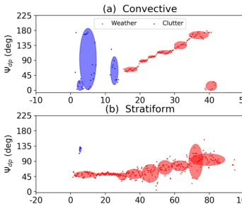
Figure 3 illustrates two examples for data masking, includ-ing a convective case (Fig. 3a) and a stratiform case (Fig. 3b). The data points in the two cases show steadily increasing trends related to anisotropic media along the wave propaga-tion path. However, between 1.3 and 15 km at an azimuth of 252◦in the convective case (Fig. 3a), the data present signifi-cant fluctuations with the minimum value at about 0◦but the maximum value at 180◦. Since the dynamic range of9dpis
from 0 to 180◦for the MZZU radar, the measurements near the ground are likely to be the clutter returns, verifying the re-sults of data masking. After 15 km, the9dppoints start from
about 50◦ and go all the way up to 180◦. Notwithstanding this trend, the points sharply decrease to about 10◦at about 40 km, indicating the occurrence of phase folding. The data masking can effectively detect the phase folding and provide valid masked data for deriving the joint PDF. On the other hand, the weather echoes are more frequently observed at 1◦ in azimuth in the stratiform case (Fig. 3b). By taking a closer look at the9dp data, we can discern that the points largely
fluctuate between 40 and 80 km due to low signal-to-noise ratio. In LR, these points may be incorrectly discarded based onσ (9dp)thresholds, leading to some missing data in the
stratiform regions. In contrast, the data masking accurately identifies weather echoes characterized by a number of verti-cally oriented density ellipses. The continuous and uniformly distributed regimes are consistent with the physical interpre-tation of stratiform precipiinterpre-tation. In addition, the data mask-ing is also sensitive to sudden jumps at the beginnmask-ing of the 9dpdata, which may be caused byδco.
4.2 9dpdensity estimation
In the previous section, it is shown that the 9dp profile
Figure 3.Examples of data masking:(a)a convective case (azimuth 252◦) and(b)a stratiform case (azimuth 1◦). The blue points and ellipses represent the clutter data and clusters, respectively, while the red color corresponds to the weather echoes. Thexaxis is the radar range in kilometers.
To estimate the relationship betweenr and9dp, we
con-siderras an independent variable, denoted asx, and9dpas a
dependent variable, denoted asy. If the minimization of the mean square error is required, the regression function is ob-tained by taking the average value ofy at fixedx, equivalent to estimating the expected values ofyconditioned onx; i.e., y(x)=E(y|x)=
Z
yp(y|x,β)dx, (10) whereβ is a set of unknown variables – for example,β= (m, w,µ,6)for the mixture model. Since the Gaussian mix-ture can be used to model any shapes of probability density with a rapid speed, the (x,y) points are then assumed to fol-low a joint PDF of Gaussian mixture, as defined in Eq. (4). Moreover, the properties of the multivariate Gaussian dis-tribution in each cluster determine the Gaussianity of the marginal distribution of either variable and the conditional distribution of one variable given the other (Bishop, 2006). Therefore, the conditional PDF ofygivenxis expressed as
p(y|x,β)=
m X
i=1
wy|xi Ny;µy|xi , 6y|xi ,with (11)
µy|xi =µyi +6yxi (6xxi )−1(x−µxi), (12) 6iy|x=6yyi −6iyx(6ixx)−16ixy, (13) wy|xi =fi(x)
f (x) =
wiN(x;µxi, 6ixx) Pm
j=1wjN(x;µxj, 6jxx)
, (14)
wherewi,µi=(µxi, µ y
i)T and6i=
6xxi 6ixy 6yxi 6iyy
are ob-tained by the EM algorithm. In Eq. (14),f (x)is the marginal PDF ofx with the parameters identical to the mixture, and fi(x) is the weighted marginal PDF of each cluster; i.e.,
f (x)=Pm
i=1fi(x). By substituting Eq. (11) into Eq. (10)
E(y|x)=
m X
i=1
fi(x)
f (x)(aix+bi),with (15) ai=6iyx(6
xx i )
−1, (16)
bi=µyi −6iyx(6ixx)−1µxi, (17)
and the conditional variance is given as (see Appendix B) σ2(y|x)=
m X
i=1
wy|xi
6iy|x+µy|xi 2
−
m X
i=1
wiy|xµy|xi !2
. (18)
Equations (15) and (18) play an important role in the joint PDF-based regression analysis, called the regression and skedastic functions (Spanos, 1999). In Eq. (15), it can be seen that the regression function in GMM consists of multiple linear kernels, which is similar to LR. However, the weighting function wy|xi is not determined by the local structure but the marginal PDF of global datax. The Gaus-sian mixture method is flexible to capture the data informa-tion, while it still retains a finite set of parameters. Moreover, Eq. (18) readily estimates the point-wise variancesσ2(y|x) that characterize the random errors in the measurements. In contrast, Eq. (3) for the LR presents the relationship between the errors σ (9dp) and σ (Kdp) under the ideal conditions,
which does not consider the random errors in 9dp. It
indi-cates that the GMM has a better error characterization based on the measurements when compared to the LR.
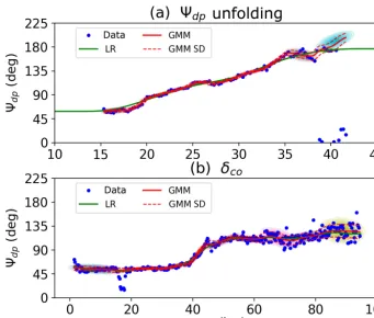
Figure 4 compares the9dpprofiles given by Eqs. (15) and
(18) with that obtained by LR. Figure 4a gives the same ex-ample as Fig. 3a, but the EM algorithm is configured dif-ferently. In the9dpdensity estimation, the mixture with full
covariance yields density ellipses of random shapes. Further-more, the algorithm repeats the fitting procedures three times to avoid the local maxima of the log-likelihood. Meanwhile, the choice of the cluster number relies on the Bayesian infor-mation criterion calculated for eachm, starting at 10 clusters. It can be seen that the mixture composed by density ellipses characterizes the data points well, since the root-mean-square error is small relative to the expected values. Between 15 and 35 km, the narrow ellipses result in9dp with a rising trend
consistent with LR. On the other hand, the mixture has very small variances, giving a high confidence for the fitted pa-rameters. From 35 km, the ellipses become wider, and the associated variances increase due to the low signal-to-noise ratio at the edge of radar echoes. What is notable, however, is that the9dpprofile dramatically increases to a large value,
whereas LR remains a relatively steady trend. It indicates the importance of the9dpunfolding for the9dpdensity
estima-tion.
Figure 4b presents another example of the density estima-tion. It is clear that the9dpprofiles produced by GMM and
LR both rise considerably along the range, and the trends for the two methods are very similar with a strong correlation of 0.998. The profile starts at about 50◦and remains relatively
stable before rising dramatically between 35 and 55 km. By 65 km,9dphas more than doubled, and then there is a steady
increase for9dp reaching about 130◦at the end of the
pro-file, which is around 70◦up on the ranges of 0 and 35 km, and 10◦more than recorded at the ranges of 55 and 65 km. If we examine9dp measured at X-band frequency, we can see
that some points fall out of the dashed lines corresponding to 1 standard error (i.e., 95 % interval). Most notably, the9dp
profile shows a sudden slump between 18 and 20 km, while theZDRcorresponds to a local peak (not shown). It may
indi-cate the occurrence ofδco. In conclusion, the expected value
and the variance of9dpcan be obtained from the joint PDF,
but the mixture needs to be tuned in terms of9dpunfolding
andδcoelimination in order to obtain the PDF of8dp.
4.3 9dpunfolding andδcoelimination
According to the continuity and consistency of the phase data, we can discern that some issues exist in the density estimation, such as ambiguous9dp andδco. Since9dp is a
range accumulative measurement of the propagation phase, depending on the initial9dp(0), the measurements may
ex-ceed the dynamic range of 0–180◦when the wave propagates through a rain medium. This situation is even more signifi-cant at X-band frequency than at S-band due to the inverse re-lation of the wavelength and the rate of phase shift. Neverthe-less, it can be noted that9dpgives a nonnegative trend along
the range for rain, and therefore the ambiguous9dpmay be
corrected accordingly (Wang and Chandrasekar, 2009). In LR, 9dp is first averaged over a small window for
weather data, and a linear fit is then performed to obtain the increment for the range gate next to the window. In the fol-lowing stage, a reference is predicted by summing up the av-erage and the increment and compared to the observed value at the same gate. If the difference between the predicted and observed values is larger than 90◦, the observed9dpis then
increased by 180◦. Finally, the correction process is itera-tively operated until the last gate.
On the other hand, the9dpunfolding is more
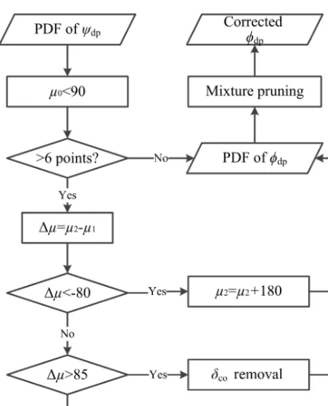
straightfor-ward in GMM. Figure 5 shows the flowchart of the9dp
un-folding and theδco elimination. After obtaining the PDF of
9dp, the initial step of the9dp unfolding selects the density
ellipses with at least six data points. Next, the second step calculates the difference of the meansµi between the two
consecutive density ellipses along the range. At this point, the PDF of9dpis ready to be corrected for ambiguous9dp.
In the final step, the mean of the latter density ellipse is added up 180◦, if the former mean is larger than the latter one by 80◦.
As illustrated in Fig. 4a, the profile9dp reaches 180◦at
interpo-Figure 4.Examples of9dpdensity estimation:(a)a9dpunfolding case and(b)aδcocase. The blue points are the9dpdata, the green curve represents the9dpprofile obtained by the linear regression model (LR), and the red curve indicates the9dpprofile produced by the Gaussian mixture method (GMM). The dashed lines are the standard deviations, while the colored ellipses show the components of the Gaussian mixture. Thexaxis is the radar range in kilometers.
lated according to the trend of the previous few gates, and the maximum value is 180◦. In contrast, the corrected
den-sity ellipses in GMM show an upward trend between 38 and 42 km, while the 9dp profile reaches a maximum value of
about 195◦, indicating the effectiveness of the9dpunfolding
in the region of heavy rain. In addition, when we apply the algorithm to a larger dataset, the rate of false alarm reaches a very small value at 0.66 %.
In addition to the ambiguous 9dp, the estimation of the
joint PDF may also be affected by nonzero δco, which is
defined as the phase difference between the horizontal and vertical polarizations upon the backscattering of the particles in a radar resolution volume. This effect occurs more fre-quently at X-band frequency than S-band due to Mie scatter-ing (Trömel et al., 2013). Theδcois shown as a sudden phase
change over a small number of gates in a monotonically in-creasing trend for rain. According to this manifestation, the magnitude and gate number of the 9dp perturbation can be
used to eliminateδco(Matrosov et al., 2002; Otto and
Russ-chenberg, 2011).
The linear regression model often adopts an iterative filter technique, which generates a new8dpprofile from either the
raw data or the filtered one based on a threshold (Hubbert and Bringi, 1995). If the filtering alters the data by 4◦, the
new profile selects the filtered data; otherwise the raw data remain. The new profile is then used as input in the next iter-ation until the convergence condition is satisfied.
As shown in Fig. 5, theδcoelimination is embedded into
the process of the9dpunfolding. For two consecutive density
ellipses, the latter density ellipse is removed if its mean is larger than the former one by 85◦. Prior to this step, the mean of the first density ellipse in the mixture should be below 90◦ to reduce theδcoeffect at the first few gates. Sinceδcooccurs
over a small number of range gates, a mixture pruning is also employed to remove the density ellipses with weights less than 0.0501, equivalent to 2 % of the data.
It is clear from Fig. 4b thatδcohas occurred at multiple
lo-cations in the data. The9dpprofile starts at a high value and
drops somewhat over the first two gates. Notably, there is a narrow gap between 18 and 20 km, while the corresponding ZDR presents a local peak. It signifies that nonzeroδco
oc-curs in this region. In GMM, these data are characterized by a density ellipse with a slightly decreasing trend, and the re-sulting expected values are consistent with the filtered data in LR. Between 70 and 90 km, a few isolated points beyond the density ellipses are associated withδco. Both of the methods
can produce8dpfollowing the main trend of the data, which
Figure 5.Flowchart of the9dpunfolding and theδcoelimination. Theµ0is the mean of the first density ellipse. Theµ1andµ2are the means of the two consecutive density ellipses along the range. Theµ1is the mean of the former one, and theµ2is the mean of the latter one.
4.4 Kdpdensity estimation
As discussed in Sect. 2.1,Kdp is the first derivative of8dp
with respect to the ranger. According to the mean value and dominated convergence theorems, the derivative of the ex-pected value of8dpconditioned onris equal to the expected
value of the derivative of8dpwith respect tor, i.e.,Kdp(see
Appendix C). Following the notation in Sect. 4.2, we denote Kdp asy0. Therefore, the expected value ofKdp is obtained
by taking the derivative of Eq. (15), yielding
E y0x
= 1 f2(x)
( m X i=1 m X j=1
fi(x)fj(x)
" x−µxj
6xxj − x−µxi
6ixx !
(aix+bi)+ai #)
. (19)
The variance ofy0conditioned onxcan be approximated by the first-order Taylor series expansion (see Appendix D); i.e.,
σ2 y0|x=E00(y|x)2σ2(y|x), (20)
whereσ2(y|x)is given in Eq. (18). By taking the derivative of Eq. (19),E00(y|x)is expressed as
E00(y|x)=2 "m
X
i=1 ai
wiy|x
0 #
+
m X
i=1
(aix+bi)
wyi|x 00
. (21)
From Eq. (C8) in Appendix C, it is clear that
wiy|x
0
= gi(x) f2(x)=
1 f2(x)
m X
j=1
fj(x)
fi(x)
x−µxj 6jxx −
x−µxi 6xxi
!
, (22)
wheregi(x)is the summation term. Subsequently, the second
derivative ofwy|xi is given as
wy|xi
00
=g
0
i(x)f (x)−2f 0(x)g
i(x)
f3(x) , where (23)
f0(x)= −
m X
j=1
x−µxj 6jxx
!
fj(x), (24)
gi0(x)=
m X
j=1
fj(x)fi(x)
x−µx i
6xxi 2
−
x−µxj 6jxx
!2
+ 1 6jxx−
1 6xxi
#
. (25)
Equations (19) and (20) are the regression and skedastic functions for theKdp estimation. In Eq. (19), it is clear that
the expected value of Kdp can be divided into two
com-ponents, including Eqs. (C7) and (C11). On the one hand, Eq. (C7) is related to the changing rateai weighted by the
marginal distribution of each cluster in the mixture, equiva-lent to a linearly weighted combination of small portions of data. If a data point is dominated by a specific cluster, i.e., the weight of a cluster is significantly larger than the others, Kdpis determined by the coefficients of the cross-correlation
and auto-correlation ofr, and independent of the means and auto-correlation of8dp, yielding a constant value within the
dominated cluster. On the other hand, Eq. (C11) shows that the weighting function also contributes to theKdpestimates
by considering the Gaussian derivative of the8dpestimates
in two or three adjacent clusters along the range. The sign of Kdpis then determined by the marginal means and variances
of the clusters, weighted by the difference of their contribu-tions to8dp.
In Eq. (20), it can be seen thatσ2(Kdp)is proportional to
σ2(8dp), which is similar to Eq. (3). When the LR is
ap-plied to the MZZU radar, we often assume thatσ (8dp)is
equal to 2.61◦with 32 pulses, 1 m s−1for Doppler spectrum and 0.98 forρhvunder the ideal conditions. However, in the
GMM,σ2(8dp)varies along the range due to the random
related to the first derivative ofKdpin Eq. (20). As the
chang-ing rate ofKdpincreases, the random errors associated with
theKdpestimates rise dramatically.
Figure 6b illustratesKdpand its variance estimated from
8dp in Fig. 6a, which is the same case as given in Figs. 3a
and 4a. It is apparent that theKdp estimates present a large
fluctuation, while the associated variances are significant. In GMM,Kdpstarts from about 0.5◦km−1and then fluctuates
between 17 and 20 km and between 24 and 42 km. In the profile, there are six local peaks with the maximum at about 8.5◦km−1. Meanwhile, theKdpvariances vary as theKdp
es-timates change. Between 15 and 17 km and between 20 and 24 km, theKdp estimates remain constant, leading to small
Kdp variances in these regions. When short excursions are
present, such as that between 18 and 20 km,Kdpvariances
in-crease significantly due to the contribution of the first deriva-tive ofKdpin Eq. (20). Furthermore, the large8dpvariances
between 35 and 42 km also result in an increase in theKdp
variances. In contrast, LR gives less fluctuation inKdp
esti-mates with two peaks at about 20 and 34 km. The compar-ison of Kdp obtained by the two methods may suggest that
a smoothing procedure is required to reduce the significant variance in GMM.
4.5 Kdpsmoothing
As discussed previously, theKdp variance is small for high
Kdp but relatively large for low Kdp. Therefore, an
adap-tive estimation is adopted in LR. For radar reflectivity (ZH)
less than 20 dBZ, the gate number nin Eq. (2) is set as 15, whilenis 8 for 20≤ZH <35 dBZ and 2 forZH ≥35 dBZ.
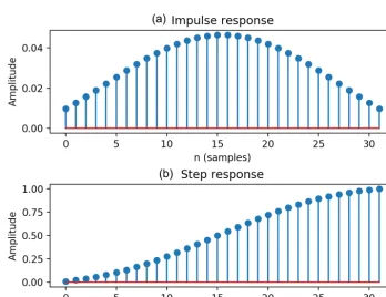
On the other hand, GMM also applies an adaptive technique based on the finite impulse filter (FIR) to the expected val-ues ofKdp in order to reduce the associated variances.
Fig-ure 7 shows the time responses of the FIR with the cutoff frequency of 0.053 and the Gaussian window of 28, which yield the best performance for the MZZU radar. The impulse response (Fig. 7a) is peaked at the center and gradually de-creases towards the two ends. Furthermore, the step response (Fig. 7b) gives the accumulation of the impulse response, in-dicating that the magnitudes around the center change faster than those at the two ends. If a longer window is required, the order of the FIR is increased accordingly. In this study, we gradually increase the order number to calculate the dif-ference between theKdp profiles obtained by the FIR filters
with two adjacent order numbers. The optimal order of the FIR filter is then set when the relative square error of the twoKdpvalues is below 0.001. For profiles with sufficiently
large data points, the order number is between 29 and 33 for the MZZU radar.
y=X
i=1
hi∗xi, (26)
where y is a smoothed data point, xi is the original data
within the smoothing window, andnis the window length. By taking the variance on both sides of Eq. (26), we have
σ2(y)=
n X
i=1
h2iσ2(xi). (27)
Therefore, the variance of the smoothed data is the weighted sum of the variances of the original data within the smooth-ing window. Since the FIR coefficients are much less than unity,σ2(y)is smaller thanσ2(x)at the same gate. Further-more, theKdp estimates with the reduced variances can be
used to reconstruct8dpto obtain smaller8dpvariances. For
a fixed gate spacing1r, the reconstructed 8dp for thejth
range gate is
8jdp=
j X
i=1
Kdpi 1rand (28)
σ2(8jdp)=
j X
i=1
σ2(Kdpi )1r2. (29)
The red curves in Fig. 6a and b illustrate the reconstructed 8dp and the smoothed Kdp using FIR, respectively. The
smoothedKdpin Fig. 6b is more consistent with the LR
re-sults compared to the originalKdp produced by the GMM.
In the first few kilometers, the smoothedKdpgradually rises
and then peaks at about 21 km. With no fluctuations, the smoothedKdp falls gradually, followed by a growth before
reaching a plateau at 33 km. After a slight decrease between 33 and 36 km,Kdp rises dramatically, which is very
differ-ent from LR. Meanwhile, the variances are small at the be-ginning but get larger asKdp is climbing. Between 20 and
33 km, theKdpestimates do not change very much, leading
to small variances in this region. But after 33 km, the vari-ances begin to increase and retain large values until the end of the profile. Overall, the smoothedKdpis stable, producing
a profile considerably consistent with LR, and the variances are significantly reduced compared to the original data. In addition, the reconstructed8dp(Fig. 6a) constantly increases
with few local fluctuations, while the associated variances are smaller than the8dpvariances in GMM.
5 Evaluation
In this section, a case study is first presented to qualitatively analyze the storm structure and evolution based onKdp. The
Figure 6.Examples ofKdpestimation:(a)8dpand(b)Kdp. The blue curves are the8dp andKdpestimates obtained by the Gaussian mixture method (GMM), the green curves represent the estimates derived from the linear regression model (LR), and the red curves indicate the reconstructed8dpand smoothedKdpprofiles (FIR). The dashed lines are the standard deviations.
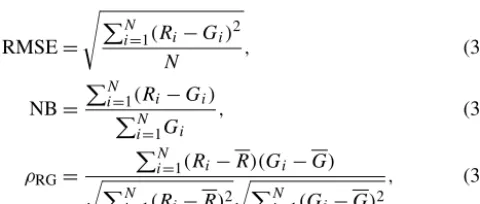
RMSE= PN
i=1(Ri−Gi)2
N , (30)
NB= PN
i=1(Ri−Gi) PN
i=1Gi
, (31)
ρRG=
PN
i=1(Ri−R)(Gi−G) q
PN
i=1(Ri−R)2 q
PN
i=1(Gi−G)2
, (32)
whereNis the sample size,Ri is the individual radar hourly
rain amount,Giis the gauge data, andRandGare the
sam-ple means for radar and gauge, respectively. The radar hourly rain amount is calculated based on the CASA radar rain-fall algorithm. It is given as (Wang and Chandrasekar, 2010; Chen and Chandrasekar, 2015)
R(Kdp)=18.15Kdp0.79, (33)
whereRis the instantaneous rain rate in millimeters per hour (mm h−1). It is noted that the radar collects instantaneous measurements every 4–5 min, whereas RGs obtain the pre-cipitation accumulations over 60 min. Therefore, it is neces-sary to average 12–15 consecutive radar scans to derive the hourly rain amounts.
5.1 Case study
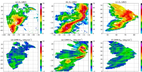
On 24 March 2016, a severe storm developed in central Mis-souri and moved eastward across Columbia, MO, causing strong winds and heavy precipitation at the surface. When the storm became mature, the S-band radars at Kansas City and St. Louis observed the storm structure at high levels, since each radar was about 150 km away from the storm. Notably, the Kansas City radar showed positive and negative Doppler velocities in a small area (not shown), indicating the occur-rence of a downburst. On the other hand, the MZZU radar il-lustrated a bow echo ofZHclose to the radar center (Fig. 8b).
In addition toZH, the GMM-basedKdp(Fig. 8d, e and f) was
also obtained to investigate the storm structure near the sur-face.
Figure 8 illustrates that the convective storm evolves from a strong and large echo to a bow shape echo and then dis-sipates at far range. At 03:04 UTC (Fig. 8a), a cell with strongZH moves into the radar area, whileKdpis moderate
with a maximum of about 3◦km−1(Fig. 8d). As the cell is
transforming to a bow shape, the radar echo becomes inten-sive and forms a rain band with embedded convective cores (Fig. 8b). It is clear to see thatKdp reaches over 10◦km−1
in these core regions (Fig. 8e), indicating very heavy precipi-tation at the surface. With the fast movement of the storm, the downburst is weaker, and the storm starts to dissipate (Fig. 8c). At 04:41 UTC, it can be seen thatKdpis gradually
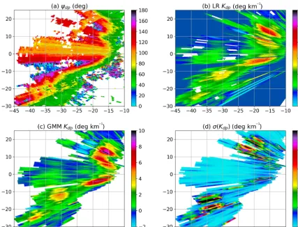
occurred at the leading edge near the echo center. The bow echo can be considered as a mesoscale convection with a hor-izontal dimension of more than 60 km. To gain further in-sight, Fig. 9 shows raw8dp andKdp for the bow echo. In
Fig. 9a, raw8dp presents large gradients along the leading
edge, rising from about 50◦to over 140◦. Due to the sharp increase,8dp exceeds the maximum dynamic range,
lead-ing to ambiguity in the areas ofX of −20 to−18 km and Y of 12 to 18 km as well as X of −40 to −23 km and Y of−8 to−5 km. In addition, the echoes behind the convec-tive cores occasionally vanish as a result of signal attenu-ation. Nevertheless, LR (Fig. 9b) produces continuousKdp
by8dp unfolding and linear interpolation according to the
trends of the profiles, but some missing data still exist within the storm, due to the low signal-to-noise ratio. In contrast, GMM (Fig. 9c) corrects these data with the expected values derived from the joint PDF and simultaneously obtains the statistical errors in the production ofKdp. It is evident that
the GMM method can efficiently handle the missing data via the mixture model, which is another advantage over the LR model. Furthermore, the statistical errors are not very large in these areas, since the missing data are filled by the distri-bution of the entire data profile. Additionally, the GMMKdp
estimates are generally a few degrees per kilometer (◦km−1) higher than the LR ones, particularly for the regions of high ZH.
By taking a closer look at GMMKdp, we can see that
the bow echo is generally characterized by Kdp of above
2.5◦km−1, while five pockets of highK
dp are identified. In
the bow head, the first pocket presents very highKdp
associ-ated with a rapid growth of8dp. Behind this pocket, there is a
region of negativeKdp, whereas LR generally yields positive
values. It may be due to a reduction of the cross-correlation coefficient caused by the low signal-to-noise ratio, since the signals have been significantly attenuated after propagating through the pocket. In the middle of the second and third pockets in the bow center, LR and GMM both show lower Kdpcompared to the two pockets, whileKdpis substantially
consistent with the gradient of8dpin the area. By
consider-ing the highZH in Fig. 8, these moderate Kdp values may
indicate less anisotropic scatterers, such as small hail in the process of wet growth. Similarly, a hail signature with maxi-mumZHof above 66 dBZ and smallKdpof 1–2◦km−1can
also be identified in the middle of the fourth and fifth pock-ets in the bow tail. Along with the expected values of GMM Kdp, Fig. 9.d depicts the statistical errorsσ (Kdp)in the
cal-culation of the expected values. The five pockets of highKdp
are generally associated with smallσ (Kdp)of a few tenths of
a degree per kilometer. However, the estimates behind the top four pockets yield very largeσ (Kdp)values with a maximum
some-Figure 8.A case study for GMM:(a)rawZH at the development stage (03:04 UTC),(b)rawZH at the mature stage (03:39 UTC), and (c)rawZH at the dissipation stage (04:41 UTC).(d),(e), and(f)are the same as(a),(b), and(c), respectively, but forKdp. The data were collected at a elevation of 0.85◦by the MZZU radar between 03:04 and 04:41 UTC on 24 March 2016.
times below 0◦km−1, such as areas ofXof−25 to−20 km andY of 11 to 20 km. In contrast, a region of highσ (Kdp)
appears in front of the bottom pocket, superimposed on the highZH area associated with hail. In conclusion, the GMM
Kdp estimates of high confidence give good agreement with
the gradients of 8dp in the leading edge of the bow echo,
while largeσ (Kdp)values are expected at the region of high
variation of theKdpestimates.
To give a further evaluation of the GMM Kdp, Fig. 10
compares the scatterplots of ZH,ZDR, andKdp to the
self-consistency (SC) relations. Referring to Park et al. (2005b), Otto and Russchenberg (2011), and Matrosov (2010), the X-band SC relations are given as
ZDR=
0 ZH≤9.5
0.051ZH−0.486 9.5< ZH≤55
2.319 ZH≥55
, (34)
Kdp=1.37×10−3×100.068ZH ×10−0.042ZDR, (35)
Kdp/Zh=1.2×10−4−4.1×10−5ZDR(ZDR<1.6), (36)
whereZH =10 logZh andZh is in mm6m−3. Figures 10a
and b illustrate that the points concentrate at the region with ZH between 10 and 40 dBZ, where the Kdp shows a low
and steady increase. Both the LRKdp and GMMKdp agree
well with the SC relation in Eqs. (34) and (35). It is notable that theKdprises dramatically from a few tenths to 8◦km−1
forZH larger than 40 dBZ. As depicted in Fig. 10a, the LR
Kdp increases greatly whenZH reaches 50 dBZ, showing a
difference from the SC relation. In contrast, the GMMKdp
in Fig. 10b gives some improvements over the LRKdp in
Fig. 10a when compared to the SC relation. Furthermore, the points ofZDR–Kdp/Zhin Fig. 10c and d may be grouped into
two clusters with high populations. The cluster with lower Kdp/Zhagrees with the SC relation in Eq. (36). On the other
hand, the clusters centered at ZDR around 0 dB are likely
caused by hails, since they are less anisotropic than raindrops with the same size. In addition, the LRKdpand GMMKdp
produce a similar distribution ofZDRandKdp/Zh, though
the distribution for the GMMKdptends to be narrower.
Moreover, the computational time is crucial for the real-time application of theKdpretrieval algorithms. For
process-ing the data in Fig. 9 in Window 10 on a PC or Linux 7 on a supercomputer, the GMM takes about 7.058/4.068 s to pro-cess theKdpwith/without the data masking, whereas the LR
reduces the time to about 2.037 s. It indicates that the LR has the advantages of simplicity and efficiency. Nevertheless, the GMM can obtain more information from the radar data, which is useful for the model studies.
5.2 Statistical analysis
In order to quantitatively evaluate the accuracy of GMMKdp,
Figure 9.Kdpestimation for the mature stage:(a)raw9dp,(b)LR-basedKdp,(c)GMM-basedKdp, and(d)GMM-basedσ (Kdp). The data were collected at 03:39 UTC on 24 March 2016.
Table 2.Statistics for the comparison between the radar and gauge. RMSE: root-mean-square error; NB: normalized bias; ρRG: Pear-son correlation coefficient; LR: linear regression model; GMM: Gaussian mixture method.
Algorithm Sites RMSE (mm) NB ρRG
LR Bradford 2.87 −0.28 0.84 Sanborn 1.97 −0.08 0.89 Auxvasse 3.25 0.21 0.67 Williamsburg 3.55 0.20 0.70
GMM Bradford 2.71 −0.31 0.84 Sanborn 2.06 −0.13 0.88 Auxvasse 3.14 0.04 0.69 Williamsburg 3.20 0.14 0.76
rain amounts, and the accompanying table (Table 2) gives the RMSE, NB, andρRGresults obtained by GMM and LR.
Consistent with the data in Table 1, the rainfall at the four sites is predominately made up of light rain with hourly rain amounts no more than 2.5 mm h−1. Nevertheless, according to Fig. 11, moderate rain with amounts between 2.6 and 8 mm h−1 provides a considerable contribution to the total
rain events, followed by a small portion of heavy rain with amounts more than 8 mm h−1. When we study the scatter-plots and statistics for each of the four sites, it is apparent that Bradford (Fig. 11a and b) and Sanborn (Fig. 11c and d) are more concentrated on the red line than Auxvasse (Fig. 11e and f) and Williamsburg (Fig. 11g and h), since Bradford and Sanborn are closer to the radar. Accordingly, RMSEs for Bradford and Sanborn (Table 2) are relatively small, about 13 %–35 % lower than Auxvasse and Williamsburg. Further-more, it can be seen that Bradford and Sanborn show neg-ative bias associated with negneg-ative NBs, indicating an un-derestimation of rain amounts by GMMKdp. In contrast, a
slight overestimation may be concluded for Auxvasse and Williamsburg by considering the point trends and the posi-tive NBs. Additionally, Sanborn claims the highestρRGout
of the four sites, yielding the best consistency between the radar and gauge.
When compared to LR statistics as given in Table 2, it is clear that GMM improves the RMSEs, NBs andρRG for
re-Figure 10.Comparison with the self-consistency relations:(a)ZHvs. LRKdp,(b)ZH vs. GMMKdp,(c)ZDRvs. the ratio of LRKdpand Zh, and(d)ZDRvs. the ratio of GMMKdpandZh, whereZH=10 log(Zh). The color scale is the number of points, and the black curves are the theoretical self-consistency relations.
mains the same. On the other hand, for Sanborn, the GMM-based RMSE has been increased and the GMM-GMM-based NB andρhv have been decreased comparing to the LR ones. It
may be due to the local complex terrain near the radar. How-ever, the difference of RMSE, NB, andρhv between GMM
and LR is a few hundredths of a millimeter, which is not sig-nificant relative to their absolute values. Overall, the rainfall estimates of GMMKdp give a better performance than that
of LR in terms of RMSE, NB, andρRGat the far ranges.
To improve the accuracy of the radar rainfall estimation, we have optimized theR–Kdprelation in terms of the RMSE
using the radar–gauge dataset. It leads to the relation as
R(Kdp)=17.33Kdp0.92. (37)
Figure 12 shows the scatterplots of the radar–gauge data and the statistics of RMSE, NB, and ρRG obtained by Eq. (37)
for all the four sites. It is clear that Eq. (37) has improved the negative trend in Eq. (33). As illustrated in Fig. 12a and b, the points give a better concentration on the one-to-one reference line with noticeable changes for higherR(Kdp). In
Fig. 12a, the LR R(Kdp)achieves fairly good RMSE, NB,
andρRGvalues at 2.30, 0.02, and 0.80, respectively. On the
other hand, the GMMR(Kdp)presents a similar distribution
to the LRR(Kdp), but the points in Fig. 12b are shifted
to-ward the vertical axis. Moreover, the GMMR(Kdp)gives
better RMSE and ρRG at 2.22 and 0.81, respectively, and
slightly worse NB at−0.03.
It can be found that the rain rates based on the GMM Kdp have a moderate consistency with the rain gauge data.
To further improve the results, some advanced rain rate al-gorithms can be considered, such as the rain–ice separation technique in the IFloodS campaign (Chen et al., 2017b) and the radar–gauge comparison method in the MC3E campaign (Giangrande et al., 2014). Nevertheless, the GMM has the advantage over the existing methods, since it can yield the variance ofKdp. Furthermore, the variance ofRcan also be
obtained by theKdp mean and theKdp variance via theR–
Kdp relation, leading to the variability in the error
Figure 11.Comparison between hourly radar and gauge data derived from GMMKdpand LRKdp.(a)GMM Bradford,(b)LR Bradford, (c)GMM Sanborn,(d)LR Sanborn,(e)GMM Auxvasse,(f)LR Auxvasse,(g)GMM Williamsburg, and(h)LR Williamsburg. The data were collected between 1 April 2016 and 2 June 2018.
6 Summary and discussions
In this study, we proposed a probabilistic method based on the Gaussian mixture model to estimate the specific differen-tial phaseKdp, which is the range derivative of the
differen-tial phase shift8dp. The Gaussian mixture method (GMM)
not only obtained the expected values ofKdpby
differentiat-ing the conditional expectation of8dp, but also yielded the
varianceσ2(Kdp)regarding the errors in the calculation of
the first derivative of8dp.
Figure 12.Same as Fig. 11 but for the optimalR–Kdprelation for the four sites.(a)LRR(Kdp)and(b)GMMR(Kdp).
of the total differential phase 9dp. The data ofr and9dp
were first fitted into a simplified Gaussian mixture to gen-erate a number of clusters, which were validated against the two sets of the σ (9dp)and σ (9dp)/σ (r)thresholds given
by radar reflectivityZH. The clusters were then combined to
form the rain cell segments, and the segments were classi-fied by comparing the weight accumulations of weather and clutter clusters. Next, the clusters within each segment were reevaluated by the thresholds according to the segment types. Finally, the azimuthally isolated points were masked out.
Secondly, the joint probability density function (PDF) was obtained by fitting the data of r and 9dp into a
mix-ture model with full covariance, where the cluster number m, weight w, mean µ, and covariance 6 were optimized via the expectation–maximization (EM) algorithm. Subse-quently, the PDF of 9dp conditioned onr was also a
mix-ture with parameters related to the joint PDF. Finally, the9dp
mean was estimated by the conditional expectation, and the statistical errorsσ2(9dp)were given by the conditional
vari-ance, which was not always constant but varied withwand the marginal PDF ofr.
Thirdly, the ambiguous9dpand backscattering differential
phase shiftδcowere corrected by examining the two adjacent
density ellipses in the mixture. On the one hand, if the former density ellipse had a mean larger than the latter one by 80◦, the latter mean was added to 180◦for9dpunfolding. On the
other hand, if the former mean was smaller than the latter one by 85◦, the latter density ellipse was removed as δco.
Moreover, forδcoelimination, the first density ellipse mean
was assumed to be below 90◦, while the density ellipses with
small weights were also removed.
Fourthly, the joint PDF ofrand8dpwas used in the
calcu-lations ofKdpandσ2(Kdp). SinceKdpwas the range
deriva-tive of8dp, the expected values ofKdp were then obtained
via the derivative of the expected value of8dp. Moreover, by
taking the first-order Taylor series expansion, σ2(Kdp)was
the product of the square of the first derivative ofKdp and
σ2(8dp), yielding nonconstant values ofσ2(Kdp).
In the final step, the expected values ofKdpwere smoothed
to reduce the associatedσ2(Kdp). An FIR filter was
imple-mented and iteratively applied to the data to search for an optimal window length. Subsequently, the reducedσ2(Kdp)
was obtained by the sum of the originalσ2(Kdp)weighted by
the FIR coefficient squares within the window. Additionally, new8dpwere reconstructed from the smoothedKdp, while
σ2(8dp)was also reduced.
The experimental results with a severe storm observed by the X-band polarimetric radar in the University of Missouri (MZZU) revealed the advantages of GMM. By studying the structure and evolution of a bow echo in the storm, it was concluded that the GMMKdp was consistent with the
gra-dients of raw8dp along the leading edge of the bow echo,
while largeσ2(Kdp)values occurred with high variation of
Kdp. The GMM method produced results similar to the LR
method, with the ability to handle the missing data. More-over, the hourly rain amounts based onKdpwere compared to
the rain gauge data, showing fairly good agreement between radar and gauge measurements. The rain amounts obtained by GMMKdpgave improvements over the linear regression
model, particularly for the far ranges.
The potential applications of GMM Kdp and σ2(Kdp)
include quantitative precipitation estimation (Cifelli et al., 2011; Chen et al., 2017a) and attenuation correction (Park et al., 2005a). For quantitative precipitation estimation, the relationship between Kdp and rain rate R is almost linear,
sinceKdp is about the fourth-order moment of the raindrop
size distribution, andR is the 3.67th-order moment. As il-lustrated in Figs. 11 and 12, theR Kdpalgorithm is
con-sistent with the in situ measurements. To further investigate theRerrors, it is necessary to consider theKdperrors in the
calculation of the first derivative of8dp. The standard
devi-ationσ (Kdp)is then related toσ (R)by a factor ofR/Kdp
(Bringi and Chandrasekar, 2001). In a similar manner,Kdpis
linearly proportional to the specific attenuationAH and
spe-cific differential attenuationADP(Bringi and Hendry, 1990).
the weather model and provide streamflow trends in the hy-drological model. In the future study, the algorithm will also be extended to other frequencies, such as the C band (Vulpi-ani et al., 2012; May et al., 1999) and S band (Bringi and Chandrasekar, 2001). The thresholds in the data masking, the 9dp unfolding, and theδco elimination will be adjusted
according to the radar specifications. Nevertheless, the steps for the calculations of the PDFs of9dpandKdpremain.
Appendix A: Regression-based estimation ofKdp Let the total differential phase 9dp bey, and let the range
gaterbex. The9dpprofile over small range segments can
be approximated by a first-order polynomial; i.e.,
y=β0+β1x+, (A1)
whereβ0andβ1are the coefficients in the linear
approxima-tion, and is an error function. It can be assumed thatis independent and individually distributed with zero mean and variance ofσ2=σ2.
In the linear regression, it is easy to find that β1=
P
i(xi−x)(yi−y) P
i(xi−x)2
, (A2)
wherex andy are the means ofxandy in the segment, re-spectively. Since
X
i
(xi−x)(yi−y)= X
i
(xi−x)yi− X
i
(xi−x)y (A3)
and X
i
(xi−x)y=y X
i
xi−N x !
=y(N x−N x)=0, (A4)
we have β1=
P
i(xi−x)yi P
i(xi−x)2
, (A5)
whereNis the number of the gates in the segment.
It is noted that the range gater is equally spaced with an interval of1r,9dp is the two-way propagation phase shift,
andKdp is the one-way specific differential phase. TheKdp
is then estimated by Kdp=
Pn
i=19dp(ri)[6i−3(n+1)1r]
n(n−1)(n+1)1r2 . (A6)
At the S band, the backscattering differential phase shiftδco
is often negligible, and thus 9dp and8dp are
interchange-able, leading to Eq. (2).
By taking the variance on both sides of Eq. (A5) and not-ingis the only variable, we have
σ2(β1)=σ2 P
i(xi−x)(β0+β1xi+) P
i(xi−x)2
, (A7)
= P
i(xi−x)2σ2 P
i(xi−x)2
2, (A8)
= σ
2
P
i(xi−x)2
. (A9)
Similar to Eq. (A6), we have
σ2 Kdp=
3σ2 9dp
1r2[n(n−1)(n+1)].# (A10)
Appendix B: Variance of8dp
We consider the rangeras an independent variable, denoted asx, and8dpas a dependent variable, denoted asy. The joint
distribution ofz=(x, y)follows a Gaussian mixture as
p(z)=
m X
i=1
wiN(z;µi,6i), (B1)
wherewi,µi, and6i are the weight, mean, and covariance
for each component, respectively. The probability ofy condi-tioned onxis also a Gaussian mixture with parameterswiy|x, µy|xi , and6iy|x, leading to the conditional expectation as
E(y|x)= Z
y
m X
i=1
wy|xi Ny;µy|xi , 6y|xi dy, (B2) = m X i=1
wiy|x Z
yNy;µy|xi , 6iy|x dy, (B3) = m X i=1
wiµy|xi , (B4)
and the second-order moment as
E(y2|x)= Z
y2
m X
i=1
wy|xi Ny;µy|xi , 6iy|xdy, (B5)
=
m X
i=1
wy|xi Z
y2Ny;µy|xi , 6iy|xdy, (B6)
=
m X
i=1
wy|xi
6iy|x+µy|xi 2
. (B7)
Therefore, the conditional variance is expressed as
σ2(y|x)=E(y2|x)−
E(y|x)2
, (B8)
=
m X
i=1
wiy|x
6iy|x+µy|xi
2
−
m X
i=1
wiy|xµy|xi !2
.# (B9)
Appendix C: Conditional expectation ofKdp