Invited Paper
Using codispersion analysis to quantify temporal changes in
the spatial pattern of forest stand structure
Case, B.S.1,∗, Buckley, H.L.2, Barker Plotkin, A.3, Ellison, A.M.3
1Department of Informatics and Enabling Technologies, Faculty of Environment, Society &
Design, Lincoln University, Lincoln, New Zealand,
2Department of Ecology, Faculty of Agriculture and Life Sciences, Lincoln University, Lincoln,
New Zealand,
3Harvard Forest, Harvard University, Petersham, Massachusetts, USA.
(Received: July 7, 2016·Accepted in final form: August 22, 2016)
Abstract
Forest development involves a complex set of ecological processes, such as dispersal and competition for light, which can generate a range of spatial patterns in forest structure that change through time. One interesting avenue of research in ecology is exploring whether spatial statistical methods can be brought to bear on such spatial patterns of forest structure to gain insight into the possible ecological processes that created them. In this study we applied a relatively new method to ecology, codispersion analysis, to investigate spatial covariation between two common measures of forest structure: tree abundance and mean basal area. We used data for four focal tree species from both a simulated and a real forest sampled at multiple time points. We assessed the significance of observed codispersion patterns using null models, in which tree diameters were iteratively and randomly reassigned to trees whose locations were kept constant. The results suggest that codispersion analysis could detect a range of spatial patterns in forest stand structure that were indicative of changing ecological processes.
Keywords:Spatial patterns·Codispersion· Forest structure·Temporal change.
Mathematics Subject Classification: 92-08.
1. Introduction
Forest development through time (“succession”) is the result of a complex interplay of factors and processes (Oliver and Larson,1996). Following a volcanic eruption, retreating glacier, logging operation, major insect outbreak, or hurricane in the forest, an initial phase of establishment of young trees at relatively high abundances ensues. The identity and or-der of species establishment in these areas is in large part determined by the interaction between the local environment, the mix of seeds dispersing into the opening, and intrinsic characteristics of different tree species, such as their tolerance to the amount of available light. For example, shade-intolerant species usually establish first and, once established, competition among individuals for light typically results in a “self-thinning” effect (Yoda
∗Corresponding author. Email: [email protected]
ISSN: 0718-7912 (print)/ISSN: 0718-7920 (online) c
et al.,1963), whereby dominant individuals outcompete smaller, nearby conspecifics, caus-ing a reduction in the numbers of trees over time and an increase in size of survivcaus-ing trees. As these stands mature, further competition among individuals of different species largely guides the trajectory of succession: shade-intolerant species typically are replaced by more shade-tolerant species. Overlain on these processes is the impact of stochastic events (e.g., insects, wind, fire), which can have profound effects on natural patterns of stand develop-ment by causing localized areas of tree mortality that interrupt and reset the otherwise directional succession (Uriarte et al.,2009). Thus, ecologists use quantitative methods to identify direct and interactive effects of successional processes and a range of disturbances that lead to observed forest structure.
One approach involves the use of spatial statistics to analyse spatial patterns of trees (Fajardo and McIntire, 2007; Kr´al et al., 2014). This approach recognizes that observed spatial patterns may be non-random, and analysis of the pattern together with associated characteristics (e.g., sizes, abundances) can reveal signatures of past ecological processes and disturbances that have shaped a given forest (Getzin et al., 2006). For example, spatial clustering of trees in a forest can arise from competitive effects, local dispersal processes, or both (Lara-Romero et al.,2015). However, spatial analyses of forest stands routinely have no temporal depth. One motivation for the work we describe here is to explore whether applying spatial methods to forest data collected through time could provide additional insights into forest dynamics (e.g., Detto and Muller-Landau, 2016; Jan´ık et al.,2016).
Figure 1. Conceptual relationships between tree abundance and mean basal area (m2) within forests. Spatial
patterns between these two variables could manifest as local areas in a forest plot where there are: A. no trees (or very few small ones); B. very few, large, dominant individuals; C. thickets of small, young trees; D. a mixture of clusters of small and large trees. The spatial arrangement of these local scenarios of tree numbers and sizes in a forest can result in relatively weak (lines 1 and 2), relatively strong (line 3), or negative abundance-basal area relationships.
throughout the plot (lines 1 and 2 in Figure 1). The relationship also may be relatively strong and positive when there is a mix of abundances and sizes distributed throughout the forest (line 3 in Figure 1). In principle, the relationship also could be negative (line 4 in Figure 1) if there is a strong spatial separation of a few, large trees and many juvenile trees of a species interspersed throughout at forest. Spatio-temporal changes in the strength or nature of the abundance-basal area relationship for a given species thus could suggest the occurrence of particular successional processes. For example, we might expect that self-thinning of a relatively homogeneous stand of juvenile trees would cause the spatial relationship between basal area and abundance to weaken as abundance decreases while the basal area of the remaining few dominant individuals increases.
We use codispersion analysis (e.g., Cuevas et al.,2013; Buckley et al.,2016a,b,c;Wang et al.,2016) to quantify temporal changes in the spatial relationships between abundance and basal area in two forest plots: one in which we simulated 200 years of forest succession following the complete mortality of a dominant species resulting from a non-native insect; and the other a real forest stand that has undergone more typical forest succession following clearcut logging in the late 1890s and damage to part of the stand in 1938. Codispersion analysis quantifies the strength, scale, and directionality (anisotropy) in the relationship between two variables that have been measured spatially either at point locations or within grid cells (Buckley et al.,2016a). We explore whether the spatial covariation in patterns of tree abundances and basal areas, examined at a number of points in time, can provide insights into successional trajectories and processes occurring in simulated and real forests. Finally, we use spatial null models (Gotelli and Graves, 1996) to test for the significance of the results and to help differentiate among possible ecological processes that underlie the observed spatial patterns (Wiegand and Moloney,2014).
2. Methods
2.1 A simulated forest
and 50, after which time no hemlock trees remained. From this simulation, we extracted for each of the four species their spatial locations and sizes (diameters), at each of six time steps (times t = 0,30,60,90,150, and 200 years). Since our initial forest conditions were fixed, stochasticity in our simulation derived from the fact that parameters for a number of the model processes (e.g., dispersal, mortality, growth) are sampled from probability distributions, leading to modest variations in outcomes of each new simulation. Here, the outcome of one representative simulation is used for subsequent codispersion analysis.
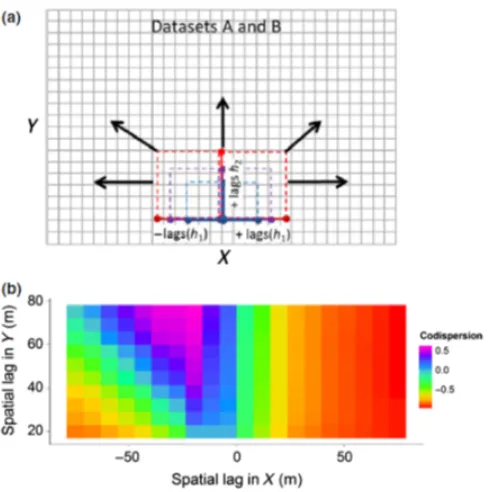
Figure 2. a) An illustration of the creation of directional spatial lags for two ecological datasets (AandB), organized as rasterized surfaces. The dashed lines represent different spatial lagshover which codispersion is calculated in different directions. (b) The codispersion graph. The color of each cell is the value of the codispersion coefficient of two variables for each given spatial laghand direction inX−Y space. Here, the graph shows negative codispersion between the two variables when computed in the east direction, but positive covariation when computed in the northwest direction, indicating anisotropy in the way in which the two variables covary. The color pattern on the graph also indicates that the two variables are most negatively correlated at spatial lags>20min the positiveX
direction, and most positively correlated at scales of c. 20−30min the negativeX direction and at c. 50−80min theY direction. Figures taken fromBuckley et al.(2016c).
2.2 The Lyford
Our second dataset comprised forest data from the Lyford plot at the Harvard Forest ( Fos-ter et al.,1999), a 2.9-ha plot situated in a maturing oak-dominated forest. Approximately 10% of this forested plot was severely disturbed by a major hurricane in 1938, after which the trees within the plot were measured and mapped on five occasions (1969, 1975, 1991, 2001, 2011). Since 1938, the Lyford plot has been undergoing typical forest succession and biomass recovery in the disturbed areas (Eisen and Barker Plotkin,2015). We extracted spatial location and DBH data for the five measurement times and for the same four tree species as were simulated with SORTIE for the Harvard Forest plot.
2.3 codispersion analysis
dataset and the five time points at the Lyford Grid plot for which data were collected in the field.
Codispersion analysis (Cuevas et al., 2013) quantifies the spatial covariation between two spatial datasets that can be in the form of point-pattern data, irregularly-spaced plot data, or data on a regular raster grid. For each of the four species, we used rasterized datasets of mean basal area (calculated from the DBH measurements of individual trees) and of tree abundance (total number of tree stems) computed within 20×20-m grid cells for the Harvard Forest plot and 5×5-m grid cells for the smaller Lyford plot.
In brief, codispersion analysis involves the application of an Epanechnikov kernel function (Cuevas et al., 2013) across all possible cell-to-cell distances for a set of spatial lags h=
{h1, h2} for each of input datasets A and B. The spatial lags comprise two vectors of
distances analysed by the kernel function: one vector of lags is oriented parallel to the x-axis of the raster, in both positive and negative lag directions, and the other vector of lags is oriented parallel to the y-axis of the raster, in the positive direction (Figure 2a). Typically, h < 0.25× the smallest plot dimension (Buckley et al., 2016b); setting h to this value reduces spurious statistical results arising from plot edge effects (Wiegand and Moloney, 2004). A set of kernel bandwidth parameters, k = {kA, kB, kAB} controls the smoothness of kernel surface generated for each input dataset and their intersection. For the rasterized dataset that we used, the distances between cells were computed from their center points.
Next, semi-variograms for A and B (γA, γB) and the semi-cross-variogram of the in-tersection of A and B (γAB), are computed for the kernel-smoothed surfaces using a Nadaraya-Watson type estimator:
b
γABk(h) =
n X i=1 n X j=1 K
h−(si−sj) k
(A(si)−A(sj))(B(si)−B(sj))
2 n X i=1 n X j=1 K
h−(si−sj) k
. (1)
Wheresis the set of spatial locations andK(·) is a symmetric and strictly positive kernel function with bandwidth parametersk (Garc´ıa-Soid´an,2007;Cuevas et al.,2013).
Finally, the empirical codispersion coefficient (Matheron,1965) is computed for each lag pairh as:
b
ρAB(h) = b γAB(h)
p b
γA(h)bγB(h)
, (2)
where bγAB is the semi-cross-variogram, bγA and bγB are the semi-variograms of the two
variables (Vallejos et al.,2015).
Results are presented as an omni-directional “codispersion graph” (Figure 2b), where codispersion variables are plotted for each combination of lags (h1, h2) in two dimensions
2.4 significance testing using null models
For both datasets, we compared the observed codispersion values to those generated under a “random labelling” null model (Buckley et al.,2016c). For each of 199 iterations of the null model, the locations of all trees in the observed data were fixed, but their diameter values were resampled randomly and without replacement, then reassigned to each tree. For each iteration, the basal areas within each grid cell in each of the rasters were then recalculated and the codispersion between abundance and basal area was re-computed. Thus, this null model kept the spatial pattern of tree locations (and their abundances) fixed, but broke the relationship between the number of trees and their sizes at the grid cell scale. We use this null model test to determine whether the spatial distribution of tree sizes is non-random, such as would occur if small trees formed clumps or thickets of recruitment and/or where large trees are over-dispersed (less likely to occur near one another).
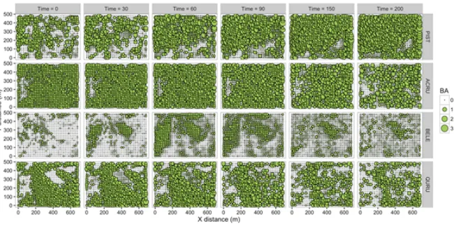
Figure 3. Scatterplots of abundance (number of individuals) and total basal area (m2) of white pine (PIST), red
maple (ACRU), black birch (BELE) and red oak (QURU) within 20×20mgrid cells in the Harvard Forest 35-ha forest dynamics plot (500×700m) at six time steps (0 to 200 years). Time = 0 represents the observed patterns at the 2014 plot measurement.
Figure 4. Total basal area (m2) of white pine (PIST), red maple (ACRU), black birch (BELE) and red oak (QURU)
Figure 5. Observed codispersion of the basal area (m2) and abundance of white pine (PIST), red maple (ACRU),
black birch (BELE) and red oak (QURU) in 20×20mgrid cells in the Harvard Forest 35-ha forest dynamics plot (500×700m) at six time steps (0 to 200 years). Contour intervals = 0.1 codispersion units.
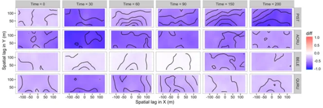
Figure 6. Observed minus expected codispersion values for white pine (PIST), red maple (ACRU), black birch (BELE) and red oak (QURU) under the random labelling model (RLM) for the Harvard Forest 35-ha forest dynamics plot (500×700m) at six time steps (0 to 200 years). The RLM keeps species distributions the same, but assigns their diameters randomly.
3. results
3.1 the simulated forest
the plot, as indicated by a change from negative to positive codispersion in a northwest direction (Figure 5: PIST,t= 200). Only minor changes in abundance or spatial pattern of stand structure occurred over the 200 years for red oak due to its long life-span and low establishment rates (Figure 5: QURU). Observed codispersion values for all species were smaller than expected under the random labelling null model (Figures 6 and 7). The one exception was for BELE at time 90 (Figures 6 and 7: BELE,t= 90), where observed and null-model codispersion values were not significantly different from random expectation at most spatial lags.
Figure 7. Null model results for the random labelling model where species distributions were kept the same, but their diameters were randomly reassigned 199 times and the codispersion between abundance and basal area 20×20m
grid cells was recalculated for white pine (PIST), red maple (ACRU), black birch (BELE) and red oak (QURU) in the Harvard Forest 35-ha forest dynamics plot (500×700m) at six time steps (0 to 200 years).
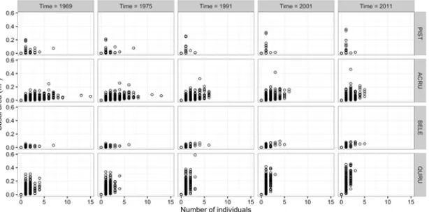
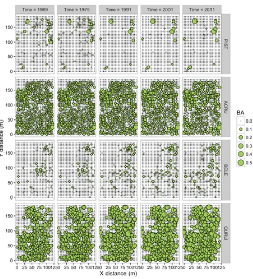
Figure 8. Scatterplots of abundance (number of individuals) and total basal area (m2) of white pine (PIST), red
maple (ACRU), black birch (BELE) and red oak (QURU) in 55mgrid cells in the Lyford Plot at five time steps between 1969 and 2011.
3.2 the lyford plot
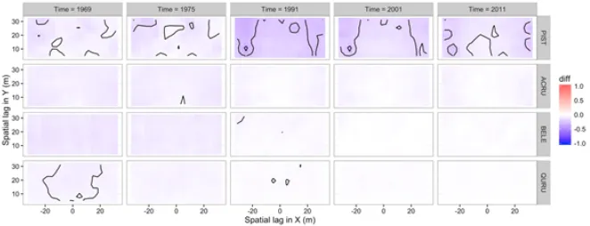
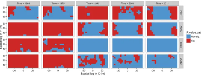
not distributed widely across the plot and, over the five sample times, decreased slightly in abundance overall but increased in basal area in those grid cells where it dominated (Fig-ures 8 and 9). There was not a clear change in observed codispersion between abundance and basal area for PIST through time, but null modelling indicated that the relationship became significantly weaker than expected at time 1991 (Figures 11 and 12); it was largely non-significant at all but the largest lags for all other times (Figure 12). There was no indication of anisotropy in codispersion relationships for any of the four species or sample times in the Lyford Plot.
Figure 9. Total basal area (m2) of white pine (PIST), red maple (ACRU), black birch (BELE) and red oak (QURU)
in 5×5mgrid cells in the Lyford plot (note that we clipped the plot so that it was a rectangle of 125×190m) at five time steps between 1969 and 2011.
4. discussion
Our two contrasting examples of forest dynamics, one of stand-level (20-m resolution) structural changes after widespread disturbance, and the other of local-scale (5-m resolu-tion) within-stand changes in an aging, relatively mature forest, suggest that codispersion analyses of species-specific, abundance-basal area relationships can illustrate a range of spatial patterns in forest stand structure and succession.
Using simulated data based on a large forest plot in which the dominant tree is rapidly declining, codispersion analysis coupled to null models clearly detected establishment and subsequent self-thinning of black birch (BELE) thickets in the relatively large gaps that were created by the loss of hemlock. The abundance-basal area relationship strengthened for BELE for the first 90 years. As the number of thickets of saplings increased, the distribution of diameters became more homogeneous across grid cells, forming a relationship resembling line 3 in Figure 1, resulting in temporally strengthening codispersion. However, this also caused codispersion to resemble that expected under a random labelling null model after time t = 90 years. Thereafter, increasing mortality of BELE individuals due to self-thinning and interspecific competition for light and space led to a more variable distribution of the locations and sizes of this species across the plot, and a subsequent weakening in codispersion between abundance and basal area. In contrast, codispersion results for white pine (PIST) and red maple (ACRU) suggested a sequence of an increasing weakening of covariation between abundance and basal area through time, and an eventual switch to a negative codispersion relationship at small spatial lags (e.g., line 4, Figure 1). This latter pattern reflects a situation in which some grid cells contain a few, large-diameter PIST and ACRU trees that have gained dominance (e.g., position B, Figure 1), whereas others contain abundant, small new recruits that are taking advantage of gaps formed by the decline of black birch (e.g., position C, Figure 1).
Figure 11. Observed minus expected codispersion values under the random labelling model for white pine (PIST), red maple (ACRU), black birch (BELE) and red oak (QURU) in 5×5mgrid cells in the Lyford plot at five time steps between 1969 and 2011. The RLM keeps species’ distributions the same, but assigns their diameters randomly 199 times.
Figure 12. Null model results for four species under the random labelling model where species’ distributions were kept the same, but their diameters were randomly reassigned 199 times and the codispersion between abundance and basal area in 5×5mgrid cells was recalculated for white pine (PIST), red maple (ACRU), black birch (BELE) and red oak (QURU) in the Lyford plot at five time steps between 1969 and 2011.
concomitantly decreasing in abundance. This process resulted in a mixture of many grid cells with no QURU trees and a few grid cells with relatively high QURU basal area, the combination of which was reflected in increasingly positive codispersion relationship at all spatial lags (e.g., line 3, Figure 1). In contrast, codispsersion of basal area and diameter of PIST weakened through time as its abundance decreased overall but a few isolated mature trees increased in their sizes (e.g., line 1, Figure 1).
acknowledgments
We acknowledge support provided to BSC and HLB as part of the Charles Bullard Fellow-ship in Forest Research program at Harvard University, and funding provided to AME, and for the Harvard Forest long term dynamics plot data collection, from the Forest GEO and Long Term Ecological Research (LTER) programs at Harvard Forest, supported by the US National Science Foundation (award number 1237491). We also thank Charlie Canham for advice on the parameterization and application of the SORTIE model, and Ronny Vallejos for useful discussions and input regarding codispersion analysis and for encouraging us to write this paper.
References
Buckley, H.L., Case, B.S., Ellison, A.M. 2016a. Using codispersion analysis to characterize spatial patterns in species co-occurrences. Ecology, 97, 32-39.
Buckley, H.L., Case, B.S., Vallejos, R., Camarero, J.J., Gutirrez, E., Liang, E., Wang, Y., and Ellison, A.M. 2016b. Detecting ecological patterns along environmental gradients: alpine treeline ecotones. Chance, 29, 10-15.
Buckley, H.L., Case, B.S., Zimmerman, J.K., Thompson, J., Myers, J.A., and Ellison, A.M. 2016c. Using codispersion analysis to quantify and understand spatial patterns in species-environment relationships. New Phytologist, 211, 735-749.
Canham, C.D., Papaik, M.J., Uriarte, M., McWilliams, W.H., Jenkins, J.C., and Twery, M.J. 2006. Neighborhood analyses of canopy tree competition along environmental gra-dients in New England forests. Ecological Applications, 16, 540-554.
Clark, J.S., Carpenter, S.R., Barber, M., Collins, S., Dobson, A., Foley, J.A., Lodge, D.M., Pascual, M., Pielke Jr., R., Pizer, W., Pringle, C., Reid, W.V., Rose, K.A., Sala, O., Schlesinger, W.H., Wall, D.H., and Wear, D. 2001. Ecological forecast: an emerging imperative. Science, 293, 657-660.
Cressie, N. and Wikle, C.K. 2011. Statistics for spatio-temporal data. Wiley, New York. Cuevas, F., Porcu, E., and Vallejos, R. 2013. Study of spatial relationships between two
sets of variables: a nonparametric approach. Journal of Nonparametric Statistics, 25, 695-714.
Dale, M.R.T. 1999. Spatial pattern analysis in plant ecology. Cambridge University Press, Cambridge.
Daley, D.J., Porcu, E., and Bevilacqua, M. 2015. Classes of compactly supported covariance functions for multivariate random fields. Stochastic Environmental Research and Risk Assessment, 29, 1249-1263.
Detto, M. and Muller-Landau, H.C. 2016. Rates of formation and dissipation of clumping reveal lagged responses in tropical tree populations. Ecology, 97, 1170-1181.
Eisen, K. and Barker Plotkin, A. 2015. Forty years of forest measurements support steadily increasing aboveground biomass in a maturing, Quercus-dominant northeastern forest. The Journal of the Torrey Botanical Society, 142, 97-112.
Ellison, A.M., et al. 2005. Loss of foundation species: consequences for the structure and dynamics of forested ecosystems. Frontiers in Ecology and the Environment, 9, 479-486. Fajardo, A. and McIntire, E.J.B. 2007. Distinguishing microsite and competition processes in tree growth dynamics: an a priori spatial modelling approach. The American Natu-ralist, 169, 647-661.
Garc´ıa-Soid´an, P. 2007. Asymptotic normality of the Nadaraya-Watson semivariogram estimator. Test 16, 479-503.
Getzin, S., Dean, C., He, F., Trofymow, J.A., Wiegand, K., and Wiegand, T. 2006. Spatial patterns and competition of tree species in a Douglas fir chronosequence on Vancouver Island. Ecography, 29, 671-682.
Gneiting, T. 2002. Nonseparable stationary covariance functions for space-time data. Jour-nal of the American Statistical Association, 97, 590-600.
Gotelli, N.J. and Graves, G.R. 1996. Null models in ecology. Smithsonian Institution, Washington.
Jan´ık, D., Kr´al, K., Adam, D., Hort, L., Samonil, P., Unar, P., Vrˇska, T., and McMahon, S. 2016. Tree spatial patterns of Fagus sylvatica expansion over 37 years. Forest Ecology and Management, 375, 134-145.
Kr´al, K., Valtera, M., Jan´ık, D., ˇSamonil, P., and Vrˇska, T. 2014. Spatial variability of general stand chracteristics in central European beech-dominated natural stands - effects of scale. Forest Ecology and Management, 328, 353-364.
Lara-Romero, C., de la Cruz, M., Escribano- ´Avila, G., Garc´ıa-Fern´andez, A., and Iriondo, J.M. 2015. What causes conspecific plant aggregation? Disentangling the role of disper-sal, habitat heterogeneity and plant-plant interaction. Oikos, 125, 1304-1313.
Ma, C. 2008. Recent developments on the construction of spatio-temporal covariance mod-els. Stochastic Environmental Research and Risk Assessment, 22, 38-47.
Matheron, G. 1965. Les variables r´egionalis´ees et leur estimation. Masson, Paris.
Oliver, C.D. and Larson, B.C. 1996. Forest stand dynamics: Update edition. Wiley, New York.
Orwig, D.A., Foster, D.R., and Ellison, A.M. 2015. Harvard Forest CTFS-ForestGEO Mapped Forest Plot since 2014. Harvard Forest Data Archive: HF253. Available online: http://harvardforest.fas.harvard.edu:8080/exist/apps/datasets/ showData.html?id=hf253.
Pacala, S.W., Canham, C.D., and Silander Jr., J.A. 1993. Forest models defined by field measurements: I. The design of a northeastern forest simulator. Canadian Journal of Forest Research, 23, 1980-1988.
R Core Team. 2014. R: a language and environment for statistical computing. R v. 3.1.2 Vienna, Austria: R Foundation for Statistical Computing. URL:http://www.R-project. org.
Uriarte, M., Canham, C.D., Thompson, J., Zimmerman, J.K., Murphy, L., Sabat, A.M., Fetcher, N., and Haines, B.L. 2009. Natural disturbance and human land use as determi-nants of tropical forest dynamics: results from a forest simulator. Ecological Monographs, 79, 423-443.
Vallejos, R., Osorio, F., and Mancilla, D. 2015. The codispersion map: a graphical tool to visualize the association between two spatial processes. Statistica Neerlandica, 69, 298-314.
Wang, Y., Pederson, N., Ellison, A.M., Buckley, H.L., Case, B.S., Liang, E., and Camarero, J.J. 2016. Increased stem density and competition may diminish the positive effects of warming at alpine treeline. Ecology 97, 1668-1679.
Wiegand, T. and Moloney, K.A. 2004. Rings, circles, and null-models for point pattern analysis in ecology. Oikos, 104, 209-229.
Wiegand, T. and Moloney, K.A. 2014. A handbook of spatial point pattern analysis in ecology. CRC Press, Boca Raton.