MODELING, SIMULATION, OPTIMIZATION
AND EXPERIMENTAL VERIFICATION OF THE
PERFORMANCE OF KA-BAND RESONANT CAP
IMPATT OSCILLATOR
TAPAS KUMAR PAL1 , J. V. PRASAD 2
Research Centre Imarat Vignyana Kancha Hyderabad – 500 069, INDIA.
J. P. BANERJEE 3
Institute of Radiophysics and Electronics University of Calcutta, Kolkata – 700009, INDIA.
Abstract:
Three dimensional modeling, simulation and optimization of a Ka-band resonant cap IMPATT oscillator has been carried out by using High Frequency Structure Simulator (HFSS) software. This model has been optimized to obtain a high quality factor at an eigen frequency of 36 GHz by varying cap radius, cap height and sliding short position. It is observed that a cap radius of 2.1 mm, a cap height of 1.46 mm and sliding short position at 0 mm and 4.5 mm leads to the desired optimization. Experiment has been carried out to study the high frequency performance of Ka-band resonant cap IMPATT oscillator with various cap diameter, cap height and sliding short position. It is observed that maximum output power at around the eigen frequency of 36 GHz is obtained when the cap diameter ranges from 3.8 – 4.2 mm and corresponding cap height ranges from 1.4 – 1.8 mm with sliding short position at 0 mm and 5.0 mm. The experimental results are in good agreement with simulation results.
Keywords: High Frequency Structure Simulator, Ka-band IMPATT oscillator, Optimization, Resonant cap.
1. Introduction
IMPact Avalanche Transit Time (IMPATT) devices based on Silicon have already been established as powerful solid-state sources for generation of high CW and pulsed power at wide range of microwave and millimeter wave frequencies [1], [2]. These devices provide high oscillator output power with high DC to RF conversion efficiency in Silicon Monolithic Millimeter Wave Integrated Circuits (SIMMWIC) [3]. The wide frequency range of operation and high power capability of IMPATT oscillator lead to its important application in mm-wave communication system and in tracking Radars. Among all the window frequencies, 36 GHz in Ka-band is gaining importance in recent years due to its wide application in civil, industrial, medical and strategic fields. In this paper the authors have carried out modeling, simulation and optimization of a Ka-band IMPATT oscillator by using High Frequency Structure Simulator (HFSS) software and the simulation results are verified experimentally.
Modeling of IMPATT oscillator involves appropriate design of the oscillator by considering its 3-dimensional behavior. This is followed by simulation and optimization of the cavity parameters with the help of HFSS software for the sake of analysis of the electromagnetic behavior of the structure. HFSS is capable of extracting basic electromagnetic field quantities, characteristic port impedances and propagation constants, generalized S-parameters and the eigen modes or resonant frequencies of the structure. HFSS has three types of solver for a particular structure which are known as DRIVEN MODAL, DRIVEN TERMINAL and EIGENMODE solvers. The authors have chosen EIGENMODE type solver for calculating the eigenmodes or resonant frequencies of the structure. The eigenmode solver also calculates the respective Quality factors of the oscillator [4].
2. Ka-band IMPATT oscillator
structures [5-6]. The resonant cap oscillator comprises a circular metallic cap placed in parallel with the broad face of the rectangular waveguide as shown schematically in Fig.1. The cap is set through a metal post into the wave guide cavity and the IMPATT diode is placed under the cap. The integrated heat sink of the diode is partially inserted into the rectangular waveguide to facilitate the optimized performance of the oscillator. The waveguide is fitted with a variable sliding short at one end while the other end is connected to the passive load. The d.c. bias current is fed to the device through a -section low pass filter. The whole system can be tuned through a sliding back short tuner. The generated microwave / mm wave signal from the IMPATT diode spreads radially outwards and is coupled to the rectangular waveguide through the open edge of the radial cavity formed between the cap and the upper plane of the integrated heat sink.
Fig.1. Schematic diagram of Ka-band resonant cap cavity
3. Modeling
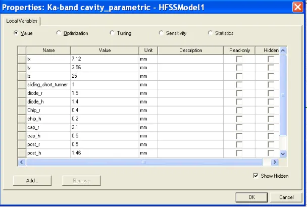
The authors have carried out modeling of the full height waveguide resonant cap structure shown in Fig.1 by using the HFSS software. The simulation and optimization of the cavity have been carried out for the optimum operation of the oscillator at 36 GHz. Three dimensional modeling of the cavity includes the rectangular waveguide cavity, the resonant cap, post, packaged IMPATT device and IMPATT diode stud. The design parameters considered in the simulation are shown in Fig. 2.
lx : width of the cavity ( in x-axis) , ly : height of the cavity (in y-axis) , lz : length of the cavity (in z-axis) , diode_r: radius of the IMPATT diode , cap_r : radius of the resonant cap , cap_h : height of the resonant cap , chip_r : radius of the chip ,chip_h : height of the chip , post_r : radius of the post , post_h : height of the post , sliding_short_tuner: position of the sliding short tuner .
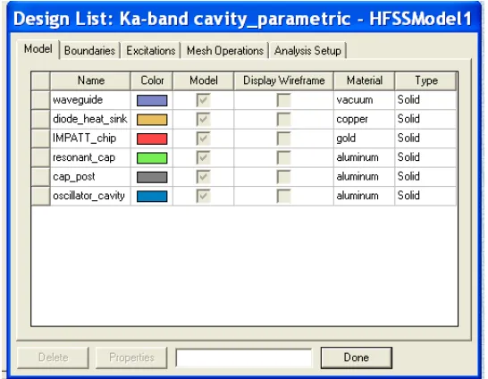
The materials used for each component in the model are very important for the modeling purpose as the physical properties of the component depend on the particular base material used. The properties of the component such as relative permeability, relative permittivity, bulk conductivity, dielectric loss tangent, magnetic loss tangent and magnetic saturation depend on the type of materials used. The cap, post and the oscillator cavity are made of Aluminium. The diode heat sink is made of copper while the IMPATT chip package is made of gold and the waveguide medium is vacuum as shown in Fig.3.
Fig 3: Snap shot of the material used in HFSS window
4. Sequential steps for 3-D Modeling of resonant cap IMPATT oscillator
A. The 3-D model of the IMPATT chip which is a cylinder of radius 0.4 mm and height 0.2 mm is created by considering a co-ordinate system with origin (0, 0, 0) as the center located at the intersection of the x-, y-, z- axes.
B. The resonant cap, which is also in the form of a cylinder, is created and cloned to the chip with a variable cap radius_r and height of 0.5 mm. The post is created with radius of 1 mm and variable post height_h. C. The cap and the post are integrated together with the diode of radius 1.5 mm and height 1.4 mm by
considering a relative ordinate system whose origin and orientation are set relative to the existing co-ordinate system.
Fig.4. Cross sectional view of the resonant cap cavity ( in HFSS window)
Fig.5. 3-D model of the resonant cap cavity(in HFSS window)
5. Solution setup
HFSS computes a solution by adding a solution setup to the design shown in Fig.6. The Solution setup consists of:
Minimum frequency Number of modes
Maximum number of passes Maximum delta frequency per pass Converge on real frequency only
Now, using different values in the solution setup, the design properties of the model are varied in order to optimize the same at a window frequency of 36GHz for maximum Quality factor.
Step: 1. The maximum frequency and the number of modes are varied and then the number of passes and maximum delta frequency per pass are also varied in order to optimize the model.
The following three parameters are varied to optimize the cavity: Cap radius (Cap_r)
Post height (Post_h) Sliding short tuner position
Fig.6. HFSS window showing the solution setup
6. Generation of HFSS Solution
For eigenmode solution type, one obtains the real and imaginary parts of the frequency and Quality factor, and also Q values for each eigenmode. The frequency column lists the real and imaginary parts of the resonant frequency for each solved eigenmode. For lossy eigenmode solutions, a Q column appears which lists the unloaded Quality factor, Q of the cavity computed for each eigenmode.
7. Calculation of Quality factor
Q is the Quality factor and is a measure of how much energy is lost in the system. Unloaded Q is the energy lost due to lossy materials. In HFSS the quality factor has been calculated as
Quality factor: (1)
In general, the quality factor has been calculated from [8]
Q = (2)*(freq)*(U/P) (2)
where,
U is the total energy stored in the cavity. P is the power lost from resistive materials etc.
8. Calculation of Resonance Frequency
The resonant frequency is the frequency of the eigenmode and calculated as
f = ( k0 C)/(2*) (3)
where,
9. Simulation and Optimization
A. The cap radius is varied from 1.8 and 2.1 mm in steps of 0.1 and optimized at each step to get a maximum Quality factor value at around 36 GHz as shown Fig.7 to Fig.10. The variation of eigen frequency vs Quality factor has been plotted in Fig.24. It is observed from the Fig. 24 that the cap radius of 2.1 mm results maximum quality factor of 15,128 at a frequency of 36.023 GHz.
B. Keeping cap radius at 2.1mm and sliding short tuner position at 0.0 mm, post height has been varied in the range of 1- 1.5 mm in steps of 0.1 and optimization is done in each step. The corresponding results are shown in Fig.11 to Fig.14. The Cap height vs eigen frequency and quality factor is plotted in Fig. 25 and it is seen that a cap height of 1.46 mm provides maximum quality factor of 61,356 at a frequency of 36.9 GHz. Further increase of cap height above 1.46 mm gives an error in the 3-D model.
C. Now, keeping both cap radius and cap height at optimized values the sliding short tuner position is varied from 0 to 5 mm in steps of 0.5. The corresponding results are in Fig. 15 to Fig. 23. The sliding short position vs eigen frequency and quality factor has been plotted in Fig.26. The optimized value of sliding short tuner position is observed at 4.5 mm with a quality factor of 39,824 at 36.8GHz.
The optimized parameters for the resonant cap IMPATT oscillator are, cap radius = 2.1 mm, cap height =1.46 mm and sliding short position = 0 mm or 4.5 mm.
24 26 28 30 32 34 36 38 40 42
0 2000 4000 6000 8000 10000 Qu ality Fa cto r [ Q ] Frequency [GHz]
22 24 26 28 30 32 34 36 38
0 2000 4000 6000 8000 10000 12000 14000 Q u ality Fa cto r [ Q ] Frequency [GHz]
Fig.7. Eigen frequency Vs Quality factor characteristic (Cap_r =1.8 mm, Post_h=1.46, S.S. tuner position = 0.0 mm)
Fig.8. Eigen frequency Vs Quality factor characteristic (Cap_r =1.9 mm, Post_h=1.46, S.S. tuner position = 0.0 mm)
22 24 26 28 30 32 34 36 38 0 2000 4000 6000 8000 10000 12000 14000 16000 Qu ality Fa cto r [ Q ] Frequency [GHz]
24 26 28 30 32 34 36 38 40 42 1000 2000 3000 4000 5000 6000 7000 8000 Q u ality Fa cto r [Q ] Frequency [GHz]
Fig.9. Eigen frequency Vs Quality factor characteristic (Cap_r = 2.0 mm, Post_h = 1.46, S.S. tuner position = 0.0 mm)
24 26 28 30 32 34 36 38 40 42 44 1000 2000 3000 4000 5000 6000 7000 8000 Q u ality Fa cto r [Q ]
Frequency [GHz] 24 26 28 30 32 34 36 38 40 42 44 0 10000 20000 30000 40000 50000 Q u ality Fa cto r [ Q ] Frequency [GHz]
Fig.11. Eigen frequency Vs Quality factor characteristic (Cap_r = 2.1 mm, Post_h = 1.0 mm, S.S. tuner = 0.0 mm)
Fig.12. Eigen frequency Vs Quality factor characteristic (Cap_r = 2.1 mm, Post_h = 1.1 mm, S.S. tuner = 0.0 mm)
24 26 28 30 32 34 36 38 40 42 0 10000 20000 30000 40000 50000 60000 70000 Qu ality Fa cto r [Q ] Frequency [GHz]
20 22 24 26 28 30 32 34 36 38 40 42 44 0 5000 10000 15000 20000 25000 Qu ality Fa cto r [ Q ] Frequency [GHz]
Fig.13. Eigen frequency Vs Quality factor characteristic (Cap_r = 2.1 mm, Post_h = 1.2 mm, S.S. tuner = 0.0 mm)
Fig.14. Eigen frequency Vs Quality factor characteristic (Cap_r = 2.1 mm, Post_h = 1.46 mm, S.S. tuner = 0.0 mm)
20 22 24 26 28 30 32 34 36 38 40 42 0 5000 10000 15000 20000 25000 30000 Qu ality Fa cto r [Q ] Frequency [GHz]
22 24 26 28 30 32 34 36 0 2000 4000 6000 8000 10000 Q u a lity Fa cto r [Q ] Frequency [GHz]
Fig.15. Eigen frequency Vs Quality factor characteristic (Cap_r = 2.1 mm, Post_h = 1.46 mm, S.S. tuner = 1.0 mm)
20 22 24 26 28 30 32 34 36 38 40 42 0 2000 4000 6000 8000 10000 12000 Q u ality Fa cto r [ Q ] Frequency [GHz]
24 26 28 30 32 34 36 38 40 42 44 -5000 0 5000 10000 15000 20000 25000 30000 35000 40000 Qu al ity Fa c tor [Q ] Frequency [GHz]
Fig.17. Eigen frequency Vs Quality factor characteristic (Cap_r = 2.1 mm, Post_h = 1.46 mm, S.S. tuner = 2.0 mm)
Fig.18. Eigen frequency Vs Quality factor characteristic (Cap_r = 2.1 mm, Post_h = 1.46 mm, S.S. tuner = 2.5 mm)
20 25 30 35 40 45 0 5000 10000 15000 20000 25000 Qu al it y F a ct or [ Q ] Frequency [GHz]
22 24 26 28 30 32 34 36 38 0 5000 10000 15000 20000 Qu ality Fa cto r [Q ] Frequency [GHz]
Fig.19. Eigen frequency Vs Quality factor characteristic (Cap_r = 2.1 mm, Post_h = 1.46 mm, S.S. tuner = 3.0 mm)
Fig.20. Eigen frequency Vs Quality factor characteristic (Cap_r = 2.1 mm, Post_h = 1.46 mm, S.S. tuner = 3.5 mm)
22 24 26 28 30 32 34 36 38 0 1000 2000 3000 4000 5000 6000 Q u ality Fa cto r [ Q ] Frequency [GHz]
22 24 26 28 30 32 34 36 38 0 20000 40000 60000 80000 100000 Q u ality Fa cto r [ Q ] Frequency [GHz]
Fig.21. Eigen frequency Vs Quality factor characteristic (Cap_r = 2.1 mm, Post_h = 1.46 mm, S.S. tuner = 4.0 mm)
10.Experimental Verification
A resonant cap IMPATT oscillator consists of a resonant cap structure under which the diode is embedded and the whole system is mounted in a rectangular wave guide. The cap along with the broad surface of the wave-guide forms a localized radial cavity around the diode. The millimeter wave power generated by the diode is coupled to the main rectangular wave-guide cavity through the vertical open edges of the radial cavity. The resonant cap can be approximated as a radial transmission line which acts like an impedance transformer between the device and the load. The cross sectional view of IMPATT oscillator used in the present study is shown in Fig.1 and the photograph of the same is shown in Fig. 27 [7]. Experimental study of resonant-cap oscillator is carried out by using a silicon Ka-band SDR IMPATT diodes having the following specifications: Frequency range = 35 – 42 GHz, Breakdown voltage = 45 Volts (max), Current = 150 mA (max), Power output = 100 mW (max). A typical spectrum (35.177 GHz) of the oscillator is shown in Fig.28.
20 22 24 26 28 30 32 34 36 38 40 42 0 10000 20000 30000 40000 Qu ality Fa cto r [Q ] Frequency [GHz]
1.80 1.85 1.90 1.95 2.00 2.05 2.10 35.6 35.8 36.0 36.2 36.4 36.6 36.8 Frequency F re qu enc y [ G H z]
Cap radius (mm)
4000 6000 8000 10000 12000 14000 16000 18000 Qu ality fa ct o r [ Q ] Quality factor
Fig.23. Eigen frequency Vs Quality factor characteristic (Cap_r = 2.1 mm, Post_h = 1.46 mm, S.S. tuner = 5.0 mm)
Fig.24. Cap radius Vs Eigen frequency and Quality factor
1.0 1.1 1.2 1.3 1.4 1.5 35.5 36.0 36.5 37.0 37.5 38.0 Frequency Fr eque nc y [G H z]
Cap height (mm)
0 10000 20000 30000 40000 50000 60000 70000 80000 Qu ality fa ct o r [Q ] Quality factor
0 1 2 3 4 5
34 35 36 37 38 39 40 41 42 Frequency Fre que nc y [ G ]
Sliding short position [mm]
0 10000 20000 30000 40000 50000 Q u ality fa ct o r [ Q] Quality factor
Fig.27. Photograph of resonant cap IMPATT oscillator Fig.28. A typical Ka-band spectrum of the IMPATT oscillator
A. Variation of Cap diameter
The cap diameter is varied from 3.4 mm to 4.5 mm and corresponding output power and frequency are measured. The results are shown in Fig.29. It is observed that the output power attains a maximum value of 90 mw for a cap diameter of 4.0 mm.
Fig.29. Variation of Output power and Frequency with Cap diameter
B. Variation of Cap height
The cap height is varied from 1 mm to 2 mm in steps of 0.2 mm and it is observed that output power increases from 52 mw to a maximum of 88 mw for a cap height of 1.6 mm and the same decreases to 72 mw for a cap height of 2 mm. The corresponding oscillation frequency varies from 36.00 GHz to 37.5 GHz.
It is also observed that maximum output power at the desired frequency (36 GHz) is obtained when the cap diameter ranges from 3.8 – 4.2 mm and corresponding cap height ranges from 1.4 – 1.8 mm. More precisely a suitable combination of the values of cap diameter and cap height i.e. 4.0 mm and 1.6 mm respectively leads to maximum output power of 90 mw at a desired frequency.
3.4 3.6 3.8 4.0 4.2 4.4 4.6 40
50 60 70 80
90 Power
O
ut
p
ut
po
w
er
[m
W
]
Cap diameter [mm]
35.5 36.0 36.5 37.0 37.5 38.0
Fr
eq
uency
[
GHz]
Fig.30. Variation of output power and Frequency with Cap height
C. Variation of Sliding short tuner position
The dependence of the oscillation frequency and output power on the sliding tuning short position has also been studied and the results are shown in Fig.31. Sliding tuning short position is varied from 0 to 9.7 mm in steps of 0.5 mm. It is observed that RF power output varies from 0 mw to 88 mw and frequency varies from 34.50 GHz to 37.75 GHz. Maximum output power is obtained at a sliding short position of 0 mm and 5.0 mm.
Fig.31. Variation of Frequency and output power with sliding short tuner position
11.Conclusion
A full height waveguide resonant cap structure has been used for realizing Ka-band IMAPATT oscillator. The resonant cap oscillator comprises a circular metallic cap placed in parallel with the broad face of the rectangular waveguide. The cap is set through a metal post into the wave guide cavity and the IMPATT diode is placed under the cap. The integrated heat sink of the diode is partially inserted into the rectangular waveguide to facilitate optimization process.
3-D Modeling, simulation and optimization of the resonant cap cavity have been carried out by using HFSS software. The effect of variation of cap radius, cap height and sliding short position has been studied by using the model and optimized for a maximum quality factor at window frequency of 36 GHz. A combination of cap radius 2.1mm, post height 1.46 mm and sliding short tuner position at 0.0 mm and 4.5mm leads to the optimum condition at the desired frequency.
1.0 1.2 1.4 1.6 1.8 2.0 50
60 70 80
90 Output power
Ou
tput p
o
wer
[m
W
]
Cap height [mm]
35.0 35.5 36.0 36.5 37.0 37.5 38.0
Fr
equency [G
Hz]
Frequency
-1 0 1 2 3 4 5 6 7 8 9 10 11
34.5 35.0 35.5 36.0 36.5 37.0 37.5 38.0
Frequency
Fr
eq
uen
cy
[GHZ
]
Sliding short tuner position [mm]
0 20 40 60 80
O
u
tp
ut pow
er
[m
W
]
Experiment has been conducted on Ka-band IMPATT oscillator with cap diameter varied from 3.4 mm to 4.5 mm and cap height varied from 1 mm to 2 mm in steps of 0.2 mm while sliding short position is varied from 0 to 9.7 mm in steps of 0.5 mm. It is observed that maximum output power at the desired frequency is obtained when the cap diameter ranges from 3.8 – 4.2 mm and corresponding cap height ranges from 1.4 – 1.8 mm with sliding short position at 0 mm and 5.0 mm .
The results obtained from the simulation have been validated by the experiment. The simulated optimized results closely match with the experimental results.
Acknowledgement
The authors1,2 are thankful to Shri. S.K. Ray, DS & Director, Research Centre Imarat, Hyderabad, Shri. R. Das, Director, RF Systems, Dr. V.G. Borkar, Head, Antenna & Components Group for their consistent support and encouragement for carrying the research work.
References
[1] Roy, S.K., “Transit Time Device”, “Encyclopaedia of Electron Devices” vol. 24, Edited by John G. Webster, Wiley & Sons, New York 1999.
[2] Banerjee, J.P., Luy, J.F. and Schaffler, F., “Comparison of theoretical and experimental 60GHz silicon Impatt diode performance, Electronic Lett. (UK) vol 27, No.. 12, pp. 1049-1051 (1991).
[3] Russer, Peter., “Si and SiGe Millimeter-wave Integrated Circuits”, IEEE Trans. on MTT, Vol. 46, No. 5, pp. 590-603,1998. [4] Ansoft HFSS user manual / guide.
[5] Howes, M. J. and Morgan, D.V., ‘Microwave Devices; Device Circuit Interactions’, A Wiley – Interscience Publication, Jhon Wiley & Sons, 1976.
[6] Gibbons, G., ‘Avalanche diode microwave oscillators’, Oxford University Press, Oxford 1973, Ch.4, pp. 45-65.
[7] Pal, Tapas Kumar., ‘A Tunable Millimeter wave (Ka-Band) IMPATT Source Using an Integrated Heat Sink cum Waveguide mount’, Patent no. 221758, INDIA, 15.02.2001.
[8] R . E. Collin , “ Foundations for Microwave Engineering”, McGraw – Hill Book Company, International Student Edition.
Authors
Shri Tapas Kumar Pal obtained his M.Sc degree in Physics with specialization in Microwaves from University of Calcutta in 1999. He has worked as a Senior Research Fellow and Senior Scientist at Centre of Advanced Study in Radiophysics & Electronics, University of Calcutta for a period of 2.5 years from Feb 2000 onwards. Later he worked as an Examiner of Patents & Designs at Patent Office, Kolkata till July 2005. Presently he is working as a Scientist ‘D’ at Research Centre Imarat, Hyderabad. He is currently engaged in development of MMW Seekers and Sensors. His special interests are Design and Development of MMW IMPATT Diodes, Oscillators and Amplifiers and their computer simulations. He has also been pursuing Ph.D (Tech) Degree at Institute of Radiophysics & Electronics, University of Calcutta, on “Millimeter wave IMPATT Diodes and Oscillators”. He is a Life Member of IETE and Member of IEEE.
Shri J. V. Prasad obtained his BE in Electronics and Electrical Engineering from Walchand College of Engineering Sangli, Maharashtra in 1984 and ME (Guided missiles) from IAT Pune in 1985. He is presently working as Sc ‘F’ at RCI and heading the division of Millimeter wave Seekers & Sensors. His areas of interest are design, development and testing of microwave and millimeter-wave antennas and their applications in seeker systems. His special interest is in MMW measurements, indoor/outdoor system calibration with simulators and millimeter wave imaging sensors & seekers. He is joint recipient of 1992 NRDC Independence day award for design and development of MMW monopulse cassegrain antenna system. He is a fellow of IETE and a member of Aeronautical society of India.