ROBUST INTERNAL MODEL CONTROL STRATEGY BASED PID CONTROLLER FOR BLDCM

ROBUST INTERNAL MODEL

CONTROL STRATEGY BASED PID

CONTROLLER FOR BLDCM

A.PURNA CHANDRA RAO* _{Y. P. OBULESU CH. SAI BABU}

EEE Department EEE Department EEE Department

Rao & Naidu Engg. College,

Ongole LBRCE, Vijayawada JNTUK, Kakinada

Abstract:

All the closed loop control system requires the controller for improvement of transient response of the error signal. Though the tuning of PID controller in real time is bit difficult and moreover it lacks the disturbance rejection capability. This paper presents a tuning of PID parameters based on internal model strategy. The advantageous of the proposed control strategy is well described in the paper. To test the validity of the proposed control, it is implemented in brushless dc motor drive. The mathematical model of brushless dc motor (BLDC) is presented for control design. In addition the robustness of the control strategy is discussed. The proposed control strategy possesses good transient responses and good load disturbance response. In addition, the proposed control strategy possesses good tracking ability. To test the effectiveness of the proposed strategy, the BLDC is represented in transfer function model and later implemented in test system. The results are presented to validate the proposed control strategy for BLDC drive.

Keywords: BLDC, IMC, PID, robustness

1. Introduction

BLDC motor is one of the permanent magnet synchronous motors also known as trapezoidal permanent magnet synchronous motor. Its applications are very wide like factory automation, transportation applications and robots etc. [1], [2]. BLDC motors possess a high accuracy of position control, involve less mechanical noise and produce less air pollution. But motors is affected by load disturbance, torque ripple and parameter variations which leads to requirement of a good controller and load disturbance compensator. In this aspect several controllers have been proposed in recent past by many researchers. Some of them include adaptive controllers, fuzzy, neural and observers etc. [3]-[7]. To tune adaptive controller, complicated on-line computations are required and online training and design experience for fuzzy and neural is required. Observer however requires large computations.

Conventional PID controllers generally do not work well for non-linear systems and particularly complex and vague systems that have no precise mathematical models. To overcome these difficulties, various types of modified conventional PID controllers were developed lately. This paper presents a simple approach to tune conventional PID controller known as Internal Model Control (IMC). The added advantage of this strategy is good tracking ability and load disturbance rejection.

Internal model control is process model approach to design PID controller parameters to obtain optimal set point tracking and load disturbance rejection. The control strategy has been used in many closed loop process control system applications. The control strategy provides a systematic procedure for PID controller compared to existing methods like Ziegler Nicholas, Cohen-coon, and Chien Hrones etc. The transformation of the synchronous machine equations from the abc variables to d, q variables forces all sinusoidal varying inductances in the abc frame to become constant in the d, q frame. Since in BLDCM back emf is non sinusoidal, the inductances do not vary sinusoidally in the abc frame and it does not seem advantageous to transform the equations to the d, q frame since the inductances will not be constant after transformation. Hence it is proposed to use the abc phase variables model for the BLDCM.

2 Materials and methods

2.1 Mathematical model of BLDCM

 

di t

 

 

 

V t =L

+Ri t + e

_b

t

dt

(1)

 

 

e

_b

t = K

_b

ω

t

(2)

 

 

T t = K i t

_t

(3)

 

dω

 

t

 

T t = J + Dω t

dt (4)

Where

V t

 

is the applied voltage,

ω

 

t

is the motor speed, L is the inductance of the stator,

i t

 

is the current of the circuit, R is the resistance of stator, e

 

t

b is the back electromotive force, T is the torque of the motor, D is the viscous friction constant, J is the moment of inertia,

Kt

is the motor torque constant and

Kb

is the back electromotive force constant.

The stator voltage can also be represented in matrix form as

L_a L L_ca

V_a R 0 0 i_{a ba} i_a e_a

V = 0 R 0 i +p L_{b b ba} L_b L_{cb b}i + e_b

0 0 R

V_c i_c L_ca L_cb L_c i_c e_c

    _{ }          _{ }          _{ }          _{ }                    _{ }    (5)

All the stator winding resistances are assumed to be equal. The back emfs have a trapezoidal shape. Further assuming no changes in the rotor reluctance with angle,

L =L =L =L_{a b c} ab bc ca

L =L =L = M

V_a R 0 0 i_a L M M i_a e_a

V = 0 R 0 i_{b b} +p M L_b M i_b + e_b

0 0 R

V_c i_c M M L_c i_c e_c

  _{ }          _{ }          _{ }          _{ }                              (6)

Since,

i = i = i = 0

a b c _,

Mi + Mi = -Mi

_b

_c

_a

The three phase stator equations become

V_a R 0 0 i_a L-M 0 0 i_a e_a

V = 0 R 0 i +p 0_{b b} L-M 0 i + e_{b b}

0 0 R 0 0 L-M

V_c i_c i_c e_c

  _{ }  _{ }      _{ }  _{ }      _{ }  _{ }      _{ }  _{ }                    (7)

And corresponding torque can be written as



e i +e i +e i

_{a a}

_{b b}

_{c c}



T =

_e

_ω

r

(8))

From the equations, the transfer function of motor can be represented as

 

  





K

ω

s

_t

=

V s

_{Ls+R Js+D +K Kt}

_b

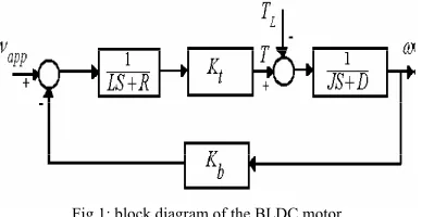
(9)

Fig 1: block diagram of the BLDC motor

In the motor, when the load torque is applied, motor speed changes drastically depending on the magnitude of the load torque. The closed loop drive acts for this change and tries to bring the speed back to normal rated value. Here, the controller is main key which keeps the drive system always in steady state.

The transfer function of the BLDC motor is obtained as follows.

 

2.726*10

5

G s =

₂

₄

s +417.7s+4.37*10

(10)

From the plant transfer function, it is evident that the system is a over damped system. Internal model control is applied to bring the closed system as under damped with less peak overshoot and zero steady state error in the step response.

2.2 INTERNAL MODEL CONTROLLER (IMC)

Since, the PID design is very difficult and is based on trial and error, PID with internal model control is proposed for brushless DC motor. IMC is based on selection of process model, which has capability to provide good performance and robust stability. IMC (internal model controller) is one of the robust controllers, which can be designed either one degree or two degree of freedom are [9, 11]. Moreover robustness can be measured based on stability and disturbance rejection [12, 13]. Fig 2 depicts the block diagram of internal model controller (IMC). From the block diagram, parameters are

Fig 2: Structure of IMC

Where , G(s) is the plant,

Gm(s) is the nominal model, R(s) is the desired valve, U(s) is the control,

D(s) is the disturbance input, Y(s) is the output and

N(s) is the measurement noise.

C(s) is called the IMC controller and is designed so that Y(s) is G(s) kept as close as possible to r(t) at all times B(s) + G(s) U(s) + D(s) + N(s) - Gm(s) U(s) =0

B(s) = (G(s) - Gm(s)) U(s) + D(s) +N(s)

Design Procedure

 Select the plant G(s).

 Partition the plant model into its minimum phase and non-minimum phase (all pass) components i.e. non-invertible and invertible. Non-invertible component Gm-(s) contains the terms, if inverted leads to instability and reliability problems, example, terms containing positive zeros and time delays. Remaining terms of the plant will be invertible Gm+(s).

 G(s) = Gm+(s) Gm-(s).

 Set the process model be Gm(s) = Gm+(s)-1

 Set Gimc(s) = Gc(s)Gf(s), where Gf(s) = 1/(1+fs)n_{. n value is chosen as order of the plant. f value shall} be selected for desired stability margins and set point tracking.

 The filter time constant must be selected the ratio of highest gain with respect to lowest gain less than

20. i.e

 

 

0

20

q

q





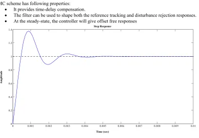
, n is chosen as 1 IMC scheme has following properties:

 It provides time-delay compensation.

 The filter can be used to shape both the reference tracking and disturbance rejection responses.  At the steady-state, the controller will give offset free responses

Fig 3: Step response of the closed loop system with IMC

The fig 3 represents the step response of the closed loop system with proposed controller. Fig 3clearly illustrates that the transient oscillation period is reduced with improving transient parameters.

2.3 Sensitivity functions and modulus margin

The sensitivity functions for a closed loop control system are described as output sensitivity functions, input sensitivity function. The sensitivity function determines the performance and complimentary sensitivity function determines the robustness. Output sensitivity function is an indicator of load disturbance rejection at the output. Output sensitivity function is defined as

KP S_yy=

1+KP (11)

-KP

S =

yb 1+KP (12)

Step Response

Time (sec)

A

m

pl

it

ud

e

0 0.001 0.002 0.003 0.004 0.005 0.006 0.007 0.008 0.009 0.01

P S_yu=

1+KP (13)

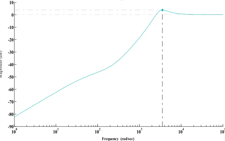
Constraints or disturbance rejections are naturally expressed in terms of frequency sensitivity shapes. The gradient of Syy at low frequency determines the dynamic behavior of the system. Each sensitivity function has its own weight age on the closed loop system. Apart from the output sensitivity function, delay margin, modulus margin and complimentary modulus margin are the new concepts defined for characterization of robust stability. The delay margin measures the minimum delay that could be added to the control loop and that provokes the destabilization of the system. This margin is particularly pertinent when the Nyquist hodograph crosses more than once the unitary radius circle. In spite of some convenient values of delay margin and phase margin, the Nyquist hodograph could pass very close to the critical point. Consequently, a relatively small insignificant modeling error could destabilize the system. This drawback is eliminated using the modulus margin concept. The modulus margin represents the smallest distance from the Nyquist hodograph to the critical point and corresponds to the radius of a circle tangent to open loop curve and having the critical point as center. In addition modulus margin can also be determined from the maximum value of Syy. In order to ensure robustness, modulus margin should be greater than 0.5 and delay margin should be higher than the sampling period. Fig 4 depicts the gain plot for the output sensitivity function.

Fig 4: Magnitude plot for output sensitivity function Bode Diagram

Frequency (rad/sec)

100 101 102 103 104 105

-90 -80 -70 -60 -50 -40 -30 -20 -10 0 10

M

ag

nitu

de

(d

B

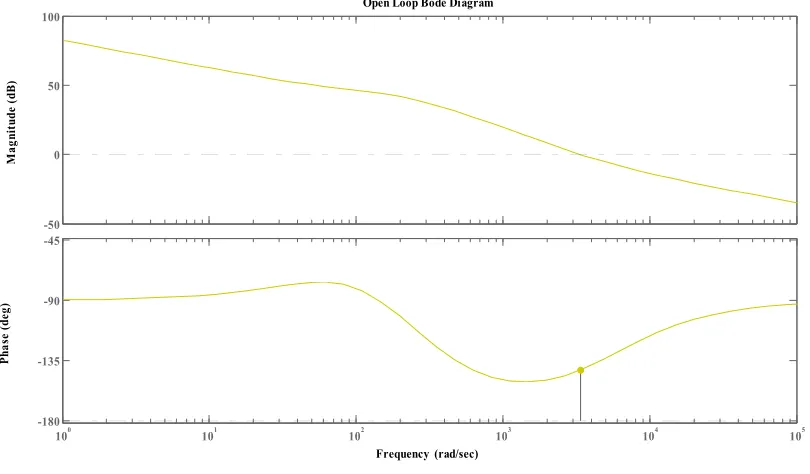
Fig 5: Gain and phase plots for system

With the proposed control, the peak gain of output sensitivity function is obtained as 3.81db (from fig 4) which corresponds to a modulus margin of 0.649. The open loop gain and phase margins as illustrated in fig 5 are GM = inf and PM = 38deg.

3

Results and Discussions

Fig 6: Simulink model of the test system

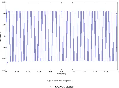
The simulation model of Closed Loop Brushless DC motor (BLDCM) Drive based on PID Controller and IMC Controller has been simulated in MATLAB/Simulink. The simulink model is represented in Fig 6. Three Hall sensors are embedded on the stator to produce six outputs. Each Hall sensors senses the magnetic flux and gives two outputs (minimum and maximum fluxes). The back emf is obtained as the difference between the maximum and minimum outputs of Hall sensor. The fig shows the back emf generation and the table depicts the truth table.

Open Loop Bode Diagram

Frequency (rad/sec)

100 101 102 103 104 105

-180 -135 -90 -45 Ph as e ( de g) -50 0 50 100 Mag ni tu de ( dB ) Reference speed (RPM) -K-rad2rpm is_a e_a v + -v + -Vdc Vab g A B C + -Te (N.m) Step Tm m A B C Permanent Magnet Synchronous Machine PID PID Controller N (rpm) emf _abc Gates Gates1 Hall emf _abc Decoder s -+ 3000

Table 1: Truth table for Hall sensor outputs and back emf

Ha Hb Hc Emfa Emf b Emf c

0 0 0 0 0 0

0 0 1 0 -1 +1

0 1 0 -1 +1 0

0 1 1 -1 0 +1

1 0 0 +1 0 -1

1 0 1 +1 -1 0

1 1 0 0 +1 -1

1 1 1 0 0 0

This simulation is based on maximum flux reading. Based on the back emf signals, respective switches in the inverter are fired so as to drive the stator of BLDC motor. The switching sequence is shown in the fig.

Table 2: Switching sequence of the inverter.

Emf a Emf b Emf c Q1 Q2 Q3 Q4 Q5 Q6

0 0 0 0 0 0 0 0 0

0 -1 +1 0 0 0 1 1 0

-1 +1 0 0 1 1 0 0 0

-1 0 +1 0 1 0 0 1 0

+1 0 -1 1 0 0 0 0 1

+1 -1 0 1 0 0 1 0 0

0 +1 -1 0 0 1 0 0 1

0 0 0 0 0 0 0 0 0

In the table, +1 indicates the entering current and -1 indicates the leaving current i.e second row indicates current enters from phase c and leaves from phase b, Hence phases b and c will be conducting. The inverter input is a controlled dc source whose magnitude is controlled by PID controller. The PID controller provides a dc voltage magnitude required depending on the error obtained by comparing the actual speed and reference set speed.

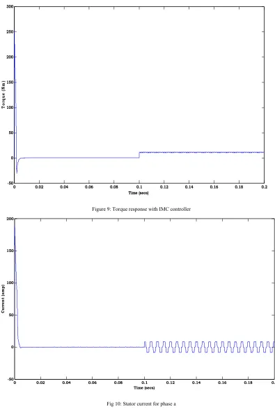
A three-phase motor rated 1 kW, 500 Vdc, 3000 rpm is fed by a six step voltage inverter. The inverter is a MOSFET bridge. A speed regulator is used to control the DC bus voltage. The load torque applied to the machine's shaft is first set to 0 and steps to its nominal value (11N.m) at t = 0.1 s.

Two control loops are used. The inner loop synchronizes the inverter gates signals with the electromotive forces. The outer loop controls the motor's speed by varying the DC bus voltage

Table 3: The test parameters of the motor taken for simulation are given below.

Parameters Value

Rated Power 1 KW

Rated Voltage 500Vdc

Resistance of the stator (R) 21.2 Ω

Inductance of the stator (L) 0.052 H

Viscous coefficient (D) 1 x 10-4_kg-ms/rad

Moment of Inertia (J) 1x10-5_kgms2_/rad

Back emf constant (Kb) 0.1433 vs/rad

Load Torque (TL ) 11 Nm

Motor Torque constant (Kt) 0.1433 kg-m/A

No of Pole Pairs 2

Speed of the rotor (N) 3000 rpm

Fig 7: simulink model of back emf generation.

The PID controller parameters are obtained from the IMC strategy. The speed and torque responses of the BLDC drive with IMC-PID controller are shown in Fig 8and Fig 9. Stator current and back emf for the phase a is shown in the figs 10 & 11.

Fig 8: Speed response with IMC controller

/ha

ha ha

/hb

hb /hc

hc /ha

/ha hb

/hb hc

/hc ha

1 emf_abc

AND AND AND AND AND AND NOT

Logical Operator1

Convert Convert Convert Convert Convert

Convert 1

Hall

0 0.02 0.04 0.06 0.08 0.1 0.12 0.14 0.16 0.18 0.2 0

500 1000 1500 2000 2500 3000 3500

Time (secs)

Sp

ee

d

(r

p

m

Figure 9: Torque response with IMC controller

Fig 10: Stator current for phase a

0 0.02 0.04 0.06 0.08 0.1 0.12 0.14 0.16 0.18 0.2

-50 0 50 100 150 200 250 300

Time (secs)

Tor

q

u

e (

N

m

)

0 0.02 0.04 0.06 0.08 0.1 0.12 0.14 0.16 0.18 0.2 -50

0 50 100 150 200

Time (secs)

C

u

rr

en

t (

am

p

Fig 11: Back emf for phase a

4 CONCLUSION

The paper presents the closed loop speed controller for the BLDC motor drive. PID parameters are tuned with internal model control strategy. . Design of Internal Model Controller is presented briefly. The transient parameters with IMC-PID are as follows:

 Peak Overshoot Mp = 37.6%

 Rise time Tr = 0.00356sec,

 Settling time Ts = 0.00336 sec,

 Peak time Tp=0.0035sec.

With the proposed IMC-PID controller, the PID parameters are: P= 38.26, I = 2112 & D = 0.0064672. From the transients’ parameters, it is observed that IMC controller gives fast response. The IMC controller is better compared to conventional PID controller as it possesses the disturbance rejection capability and can withstand to load fluctuations. Modulus margin for the IMC-PID controller is 0.649, which indicates a good robustness. The torque response clearly indicates the effectiveness of IMC. As seen from the torque curve, torque ripples are minimized with IMC-PID. PID tuning with IMC is very easy as only one parameter has to chosen.

5

REFERENCES

[1] V. Tipsuwanporn, W. Piyarat and C.Tarasantisuk, “Identification and control of brushless DC motors using on-line trained

artificial neural networks,” in Proc. Power Conversion Conf., pp. 1290-1294, Apr.2002.

[2] Atef Saleh Othman Al-Mashakbeh “Proportional Integral and Derivative Control of Brushless DC Motor” European Journal of

Scientific esearchVol.35 No.2 (2009), pp.198-203

[3] Microchip Technology, “Brushless DC (BLDC) motor fundamentals”, application note, AN885, 2003.

[4] Gwo-Rueyyu and Rey-Chue Hwang “Optimal PID Speed Control of Brushless DC Motors Using LQR approach” IEEE

International Conference on systems, Man and Cybernetics, 2004, pp.473-478.

[5] C. Gencer and M. Gedikpinar “Modeling and Simulation of BLDCM using Matlab/Simulink” Journal of Applied Sciences

6(3):688-691, 2006.

[6] Allan R. Hambley, “Electrical Engineering Principles and Application”, Prentice Hall, New Jersey 1997. [7] Rivera, D.E.skogestad, S.Morari M.IMC 4: PID controller design. Ind.Eng chem..Process des. Dev 1986, 25,252.

[8] Gaddam Mallesham, Akula Rajani ,”Automatic Tuning of PID Controller using Fuzzy Logic”, Internal Conference on

Development and Application Systems,2006,pp.120-127,

[9] K. Ang , G.Chong, and Y. Li, “PID control system analysis, design, and technology,” IEEE Trans.Control System Techno

gy,vol.13,pp.559-576,July 2005.

[10] Bergh, L.G. MAC Gregory. J.F. constrained minimum variance- Internal model structure and robustness properties.IND. Eng

chem. Res.1986, 26, 1558.

[11] Chein, L-L Fruehauf, P.S consider IMC tuning to improve controller performance. Chem. Eng. Prog 1990, 86,33.

0 0.02 0.04 0.06 0.08 0.1 0.12 0.14 0.16 0.18 0.2 -300

-200 -100 0 100 200 300

Time (secs)

B

ack em

f (

[12] N.Mohan, T.M.Undeland, and W.P.Robbins, Power Electronics Converters, Applications, and Design, New York: John Wiley & Sons, 1995.

[13] K.Ogata, Modern Control Engineering, New Delhi, India: Prentice-Hall of India Pvt Ltd., 1991.

Biography

A.Purna Chandra Rao received the B.E (Electrical and Electronics Engineering) degree from Andhra University, Visakhapatnam, India, M.Tech degree from Jawaharlal Nehru Technological University, Anantapur, India in 1998 and 2004 .He is currently working as an Associate Professor in the Dept. of Electrical and Electronic Engineering, at Rao & Naidu Engineering College, Ongole. His area of interest is Power Electronics, and Electrical Drives.

Y. P. Obulesu received his B.E degree in Electrical Engineering from Andhra University, Visakhapatnam, India, M.Tech degree from Indian Institute of Technology, Kharagpur, India, in 1996 and 1998.He received his PhD degree from Jawaharlal Nehru Technological University, Hyderabad, in 2006. He has published several National and International Journals and Conferences. His area of interest is the simulation and design of power electronics systems, DSP controllers, fuzzy logic and neural network application to power electronics and drives.