Research article Available online www.ijsrr.org ISSN: 2279–0543
International Journal of Scientific Research and Reviews
Estimation of Autocorrelation function and partial Autocorrelation
function of Evapotranspiration for Ranchi district, India, in context of
time series Modelling.
Gautam Ratnesh
*1and Sinha Anand Kumar
21
Department of Civil and Environmental Engineering, Birla Institute of Technology, Mesra-835215, India. E-mail: [email protected]
2
Department of Civil and Environmental Engineering, Birla Institute of Technology, Mesra-835215, India. Email: [email protected]
http://doi.org/10.37794/IJSRR.2019.8403
ABSTRACT
Auto correlation function (ACF) and Partial Auto correlation function(PACF) play important
role in time series analysis. In this study ACF &PACF for reference crop evapotranspiration have
been found. The data series of 102 years (1224 months) of Ranchi district are used for determination
of ACF and PACF. This study is helpful for calculating parameters of different time series modelling
like autoregressive (AR) Model, moving average (MA) Model, autoregressive moving average
(ARMA)model, autoregressive integrated moving average (ARIMA)model, etc. Apart from that,
these are also helpful for time series analysis of different data series of numerous fields. The study is
beneficial for, Researcher in the field of hydrology, statistics, econometrics, big data series,
predictions of sales in corporate field, forecasting of rainfall, temperature, to see the pattern of
climate change, etc.
KEY WORDS: ACF, PACF, evapotranspiration, autoregressive, moving average
*
Corresponding author
Ratnesh
Gautam
Ph.D. Research Scholar,
Department of Civil and Environmental Engineering,
1.
INTRODUCTION
Autocorrelation means correlation of time series with its own past and future values.
Autocorrelation is also denoted by serial correlation or lagged correlation, which indicate correlation
between numbers of series of time dependent. Auto correlation may be positive or negative. Positive
autocorrelation may be considered a particular form of persistence. Autocorrelation may be
predictable, probabilistically, because future values depend on current and past values. There are
three important tools for assessing the autocorrelation of a time series i.e. time series plot, the lagged
scatter plot, the autocorrelation function. The partial autocorrelation function can be defined as
regression of the series against its past lags. Generally, PACF helpful for possible order of
autoregressive term and ACF confirming moving average term. Evapotranspiration is the important
component of water cycle. Correct analysis of evapotranspiration is challenge for researcher and
hydrologist to see the climate change. For analysis of evapotranspiration numbers of equations and
formulas are given by different researchers. Present study is helpful for stochastic analysis of
evapotranspiration. Mohan et al.1 determined autocorrelation function and partial auto correlation
function for forecasting weekly reference crop evapotranspiration series. Etuk et al.2 used
autocorrelation and partial auto correlation for modelling monthly Uganda shilling /US dollar
Exchange rate by seasonal box-Jenkins techniques. Popale et al.3 applied autocorrelation and partial
autocorrelation function for stochastic generation and forecasting of weekly rainfall for Rahuri
region. Jafri et al.4 applied auto correlation and partial auto correlation function for stochastic
approaches for time series forecasting of rate of dust fall. Helmy et al.5 calculated auto correlation
and partial autocorrelation for estimating monthly reference crop evapotranspiration in Najran
region, KSA, using seasonal regression autoregressive model. Posilovikos et al.6 used auto
correlation function and partial auto correlation function for forecasting of remote sensed daily
evapotranspiration data over Nile Delta Region, Egypt. Dabral et al.7 determined auto correlation
function and partial auto correlation function for time series modelling of pan evaporation a case
study in the northeast India. Hamdi et al.8 calculated auto correlation function and partial auto
correlation function for developing reference crop evapotranspiration time series simulation model
using class a pan, a case study for the Jordan valley Jordan. Asadi et al.9applied auto correlation
function and partial auto correlation function for forecasting of potential evapotranspirat ion using
time series analysis in humid and semi humid regions. Medelisation et al.10 determined sample
partial autocorrelation function of a multivariate time series. Trajkovic11 used auto correlation
function and partial auto correlation function for comparison of prediction models of reference crop
integrated model of auto correlation function and neural network. Gorwantiwarret al.13 forecasting of
Evapotranspiration for Makni Reservoir in Osmanabad District of Maharashtra, India using
autocorrelation function and partial autocorrelation function.The main goal of this study is to
determine correct value of auto correlation function (ACF )and partial auto correlation function
(PACF) for reference crop evapotranspiration.
2.
MATERIAL AND METHOD
Study area Ranchi district is the capital district of Jharkhand state of India, which is situated at
latitude 23.35˚N, Longitude 85.23˚E,the geographical area is approximately 5231 sq.km.Elevation
from the mean sea level is 2140 ft, annual rainfall is 1530mm of rainy, winter, summer seasons. The
main minerals are lime stone, coal, asbestos and ornamental stones etc. and crops are rice, millets,
pulses and oil seeds. The total population is around 2912022. Data series is taken from the same
Ranchi district. A autocorrelation function is a bar chart of correlation coefficients between the given
series and its lags. The partial autocorrelation function is the bar chart of partial correlation
coefficient between the given data series and its lags. If Y variable is regressing on variable
X1,X2,and X3, then the partialCorrelation between Y and X3 is not determined by their relations
with X1and X2.This correlation can be determined as the reduction in variance square root , which is
computed by adding X3 to the regression of Y on X1 and X2.The autocorrelation of a Y time series
at lag1 is the correlation coefficient between Yt and Yt-1, which is also correlation between Yt-1 and
Yt-2.In a series, if partial autocorrelation function shows sharp cutoff whereas autocorrelation
function decays more slowly, that series represent AR signature, and if vice-versa then MA
signature.The autocorrelation function (ACF) is widely known for identifying the presence of serial
correlation.
Mathematical expression of the autocorrelation function for the series y1, y2, , yn, the sample autocorrelation at lag k is
∑ ̅ ̅ ∑ ̅
[1]
Where ̅ ∑
The standard error of rk is
∑
[2]
The limits for the values of the ACF are given by
√ ,Where z1-α/2 is the standard normal deviate
for 1-α/2 level of confidence (usually 95% level of confidence and the value for Z =1.96).
The sample partial autocorrelation at lag k is
r11 = r1 [3]
r22 = (r2 –r12)/ (1-r12) [4]
rkj = rk-1,j- rkk rk-1, k-j , k = 2,…., j = 1,2,…..,k-1 [5]
rkk =
∑ ∑
, k=3,……. [6]
Where rkj = rk-1,j – rkk. rk-1, k-j
The limits for the values of the PACF are given by
√ ,Where z1-α/2 is the standard normal deviate for 1-α/2 level of confidence (usually 95%
level of confidence and the value for Z =1.96).
Q is the Box- LjungStatistics , the equation of Q value is-
Qk=n(n+2)∑
[7]
In case of n is large ,Qkhas the chi-square distribution having degree of freedom of freedom k-p-q,
where p is the autoregressive operator and q is the moving average operator.
In any time series study the pattern of autocorrelation is modelled, for itself, in preparation for test of
intervention, forecasting. To check the linear or quadric pattern in data series, effect of previous
value to the current one. Due to rotation of sun, seasonal pattern occur in the data series, the data
series are examined for the seasonality.
3.
DATA COLLECTION AND ITS ANALYSIS
The data series is collected from „http://indiawaterportal.org/met data. To know the properties
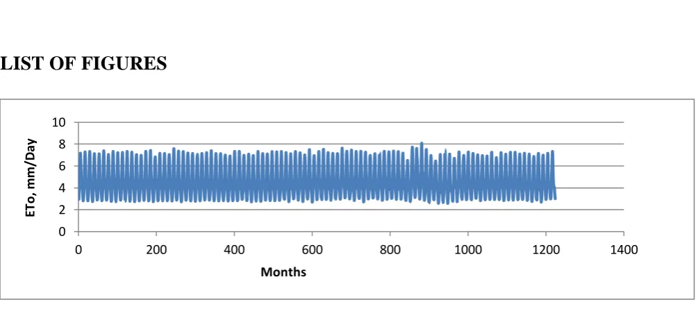
of data, it is plotted on the simple graph at excel sheet. Figure1 shows there are no trends in data
series but there is strong periodicity. For time series analysis, the data should be free from
periodicity. Figure 2 is the plot of seasonally differenced data series with no periodicity. For making
data series stationary, seasonal differenced data is re differenced by difference of one month. Figure3
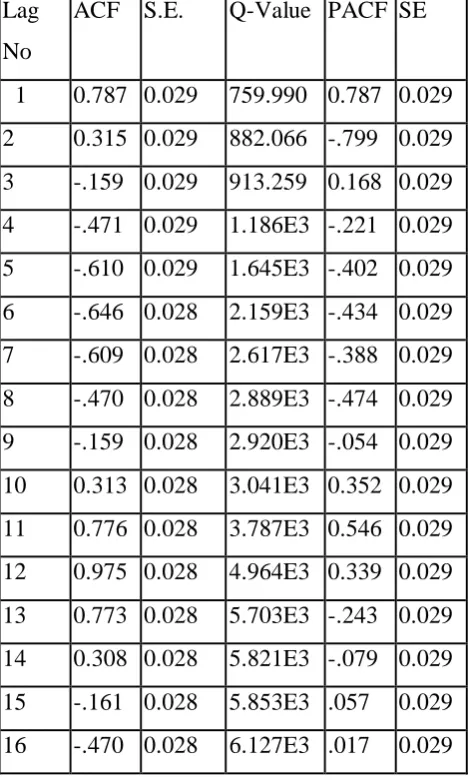
and PACF SPSS16 Software was used. Table1 shows autocorrelation functionand partial
autocorrelation of evapotranspiration data series at lag16. Standard error and L-jung statistics
(Q-value) is also located corresponding to the autocorrelation and partial autocorrelation values. Table 2
shows autocorrelation and partial autocorrelation of seasonally differenced evapotranspiration data
series at lag16. Table3 has the numerical values of autocorrelation and partial autocorrelation
function of seasonally and non- seasonally differenced evapotranspiration data series at lag 16.Figure
4
to Figure 9 shows plots of autocorrelation function and partial autocorrelation function
corresponding to the numerical values of Table1, Table 2and Table 3.
4.
RESULT AND DISCUSSION
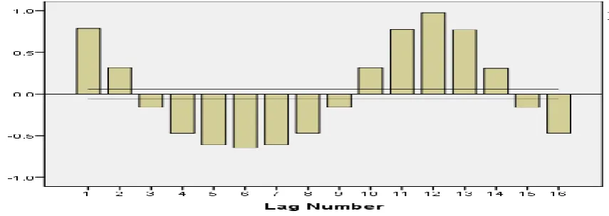
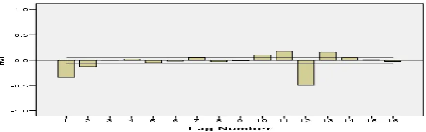
Figure 4 and Figure 5 represents autocorrelation function and partial autocorrelation function
at 16 lags and 95% confidence limit respectively. The patterns of spikes shows cyclic pattern in the
data series. Figure 6 and Figure 7 shows auto correlation function partial auto correlation function of
seasonally differenced data series respectively at lag16. In this figures autocorrelation function is
slowly decay whereas partial autocorrelation function shows sharp cut off, this indicate presence of
autoregressive(AR) in the data series. Figure 8and Figure9 shows autocorrelation and partial
autocorrelation of seasonally and non-seasonally differenced data series at lag 16. In these figures
autocorrelation function shows sharp cut off and autocorrelation function decay slowly, this indicate
presence of moving average (MA) in the data series.In this way on the basis of spikes appear in the
figure of autocorrelation and partial autocorrelation, the presence of AR, MA are identified. These
finding are beneficial for different time series modelling like autoregressive(MA) model, moving
Average(MA) model, autoregressive moving average(ARMA)model,autoregressive integrated
moving average(ARIMA) model etc. Randomness in data can also be checked by autocorrelation
function at time lags. Autocorrelation also check, relationship of observation to the adjacent
observation, white noise condition of observation, sinusoidal properties of data series,and appropriate
model for the time series.
5.
CONCLUSION
This paper is inspired by conjecture that evapotranspiration series would contain little amount of
autocorrelation, but persistent for different lags.Data series did not show any inherent trends, but
show strong periodicity. Auto correlation function and partial autocorrelation are determined upto
lags 16. Autocorrelation function and partial autocorrelation have both negative and positive values.
As per requirements lags of auto correlation function and partial autocorrelation can be changed.
average modelling.Auto correlation function and partial autocorrelation may also be applying for
prediction and forecasting purposes. They gives autoregressive or moving average present in the
models.The presence of autocorrelation and partial autocorrelation is evapotranspiration data is
important, because for modelling and forecasting of evapotranspiration, the regression model assume
that error terms should free from autocorrelation, when autocorrelation is present, the regression
model is misidentified. So alternative model may produce a better modelling and forecasting of
evapotranspiration.
REFERENCE
1. Mohan, S. and Arumugam, N. “Forecasting weekly reference crop evapotranspiration series”
Hydrol. Sci. 1995;40(6):689-702.
2. Etuk,E.H., and Natamba, B., “Modelling monthly Uganda shilling /US dollar Exchange rate
by seasonal box-Jenkins techniques” , International journal of life science and engineering,
2015;1(4):165-170.
3. Popale, P.G.andGorantiwar, S.D., “Stochastic Generation and Forecasting of Weekly Rainfall
for Rahuri Region.,International Journal of Innovative Research in Science,Engineering and
Technology, 2014; 3(4):14.
4. Jafri , Y.Z. (2012), “Stochastic approaches for time series forecasting of rate of dust fall”,
International journal of physical sciences, 23 january.2012; 7(4):676-686.
5. Helmy, A.,and Dahim,M.A., “estimating monthly reference crop evapotranspiration in Najran
region , KSA, using seasonal regression autoregressive model.” , International conference on
civil, biological and environmental engineering, May 2014; 27-28.
6. Psilovikos,A., and Elhag, M., “Forecasting of Remotely Sensed Daily Evapotranspiration Data over Nile Delta Region,Egypt”, Water Resources Management, 2013;27:4115-4130
7. Dabral, P.P. , Jhajharia, D., Mishra, P., Hangshing, L. and Doley B.J., “Time series modelling of pan evaporation a case study in the northeast India.” Global NEST Journal, 2014; 16(2):
280-292
8. Hamdi, M. R., Bdour, A.N. and Tarawneh A.N., “Developing reference crop
evapotranspiration time series simulation model using class a pan: A case study for the
Jordan Valley, Jordan”, Journal of Earth and Environmental Sciences. 2008;1(1): 33-44.
9. Asadi A., Vahdat S. F. and Sarraf A., “The forecasting of potential evapotranspiration using time series analysis in humid and semi humid regions”, American Journal of engineering
10. Modelisation, L. D. ,Calcul, Grenoble, and France, “ Sample partial autocorrelation function
of a multivariate time series”, Journal of multivariate analysis, 1994;50:294-313.
11. .Trajkovic, S., “ Comparison of prediction models of reference crop evapotranspiration” , the
scientific Journal factauniversitatis, 1998;1(5):617-625.
12. Abolfazli, H.,Asadzadeh, S.M.,Shirkouhi, S.N.,Asadzadeh, S.M., and Rezaie, K., “forecasts
rail transport petroleum consumption using an integrated model of auto correlation function
and neural network”,acta polytechnic hungerica., 2014;11(2):2014.
13. Meshram,D.T.,Gorantiwar, S.D., Kulkarni, A.D. and Hangargekar, P.A. “Forecasting of Evapotranspiration for Makni Reservoir in Osmanabad District of Maharashtra, India”,
International Journal of Advanced Technology in Civil Engineering, ISSN:2231-5721, 2013;
2(2):23.
LIST OF FIGURES
Figure1 time series plot of reference crop evapotranspiration (ETo)
Figure 2. Graph of the Seasonally Differenced Eto(Sdiff.Eto) Data Series( Difference of 12 months)
0 2 4 6 8 10
0 200 400 600 800 1000 1200 1400
ET
o
, m
m
/D
ay
Months
-8 -6 -4 -2 0 2 4
0 200 400 600 800 1000 1200 1400
ET
o
,m
m
/D
ay
Figure 3. Graph of Seasonally and then non- seasonal differenced Eto (Nsdiff.Eto) data series(Differenced of one
month)
Figure 4 Autocorrelation function (ACF) plot at 16 Lags.
Figure 5 Partial autocorrelation function (PACF) plot at 16 lags
-4 -2 0 2 4
0 200 400 600 800 1000 1200 1400
ET
o
, m
m
/D
ay
Figure 6.Autocorrelation function (ACF) plot of seasonally differenced data at 16 Lags.
Figure 7.Partial autocorrelation function (PACF) plot of seasonally differenced data at 16 Lags.
Figure 9. Partial autocorrelation function (PACF) plot of seasonally and non- seasonally differenced data at 16
Lags.
Table1. Autocorrelation function (ACF) and partial autocorrelation function(PACF) at 16 lags
Lag
No
ACF S.E. Q-Value PACF SE
1 0.787 0.029 759.990 0.787 0.029
2 0.315 0.029 882.066 -.799 0.029
3 -.159 0.029 913.259 0.168 0.029
4 -.471 0.029 1.186E3 -.221 0.029
5 -.610 0.029 1.645E3 -.402 0.029
6 -.646 0.028 2.159E3 -.434 0.029
7 -.609 0.028 2.617E3 -.388 0.029
8 -.470 0.028 2.889E3 -.474 0.029
9 -.159 0.028 2.920E3 -.054 0.029
10 0.313 0.028 3.041E3 0.352 0.029
11 0.776 0.028 3.787E3 0.546 0.029
12 0.975 0.028 4.964E3 0.339 0.029
13 0.773 0.028 5.703E3 -.243 0.029
14 0.308 0.028 5.821E3 -.079 0.029
15 -.161 0.028 5.853E3 .057 0.029
Table 2. Autocorrelation function (ACF) and partial autocorrelation function (PACF) of seasonally difference
evapotranspiration data at 16 lags.
Lag No ACF SE Q- Value PACF SE
1 .388 .029 182.478 .388 .029
2 .189 .029 226.013 .046 .029
3 .159 .029 256.683 .084 .029
4 .125 .029 275.859 .038 .029
5 .062 .029 280.478 -.017 .029
6 .057 .029 284.376 .023 .029
7 .077 .029 291.603 .043 .029
8 .032 .029 292.832 -.024 .029
9 .021 .029 293.349 .003 .029
10 .018 .029 293.757 -.002 .029
11 -.106 .029 307.549 -.143 .029
12 -.444 .029 549.083 -.443 .029
13 -.178 .029 588.004 .164 .029
14 -.103 .029 601.111 .001 .029
15 -.090 .029 611.110 .035 .029
16 -.089 .029 620.882 -.007 .029
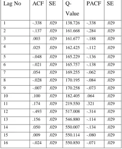
Table 3 .Autocorrelation function (ACF) and partial autocorrelation function (PACF) of seasonally and non-
seasonally difference evapotranspiration data at 16 lags.
Lag No ACF SE Q-
Value
PACF SE
1 -.338 .029 138.726 -.338 .029
2 -.137 .029 161.668 -.284 .029
3 .003 .029 161.677 -.188 .029
4 .025 .029 162.425 -.112 .029
5 -.048 .029 165.229 -.136 .029
6 -.021 .029 165.757 -.138 .029
7 .054 .029 169.255 -.062 .029
8 -.028 .029 170.195 -.084 .029
9 -.007 .029 170.258 -.073 .029
10 .100 .029 182.405 .064 .029
11 .174 .029 219.550 .321 .029
12 -.493 .029 517.008 -.314 .029
13 .156 .029 546.880 -.114 .029
14 .050 .029 550.007 -.134 .029
15 .009 .029 550.114 -.080 .029