Complex photonic structures for energy efficiency
M. BurresiandD. S. Wiersma
European Laboratory for Non-linear Spectroscopy (LENS), University of Florence Via Nello Carrara 1, 50019 Sesto Fiorentino (FI), Italy
Istituo Nazionale di Ottica (CNR-INO) - Largo Fermi 6, 50125 Firenze, Italy
Summary.— Photonic structures are playing an increasingly important role in energy efficiency. In particular, they can help to control the flow of light and improve the optical properties of photovoltaic solar cells. We will explain the physics of light transport in such structures with a special focus on disordered materials.
1. – Introduction
The quest for efficient harvesting of solar radiation is extremely relevant in the re-newable energy field. Research has an interdisciplinary character, ranging from material science [1-6] to optics [7,8] and nanophotonics [9-13]. Particular attention is dedicated to the so-called third-generation solar cells, among which thin-film technologies provide a promising alternative to standard silicon cells or to cells based on sometimes very expen-sive and rare, materials (e.g., CdTe, CIGS) [4]. Due to the reduced thickness of these thin films (even below 1μm), strategies to increase their performances can play an important role. Different approaches can be followed amongst which the design and fabrication of engineered photonic structures. This can either lead to enhanced absorption, or can reduce the amount of required material and hence reduce fabrication costs.
C
Nanophotonics offers interesting possibilities for improving solar cell absorption [14-16]. Standard optics is limited by an upper thermodynamical limit [17], which can however be surpassed by nanophotonic strategies in particular when the absorbing films are extremely thin [18]. Through different photonic architectures it is possible to aug-ment the optical absorption by, for instance, trapping light within ultra-thin films [14], or even manipulate the photon density of state [15] or slowing down light in absorbing thin films. This can be achieved by periodic photonic structures [14, 15] or disordered ones [19-21], as it has been recently proposed in a two-dimensional system [22] in which disorder modes are on the verge of light (Anderson) localization [23-25].
In these proceedings we will focus on the optics of disordered systems. Disorder can slow down transport or increase the path length of light inside a material, and thus significantly increasing the probability of light to be absorbed. Different degrees of disorder can be used to control the transport. Also, different dimensions of the disordered system give rise to significantly different optical properties, providing a variety of possible strategies, depending on the specific geometries of the system.
2. – Multiple scattering for controlling light propagation
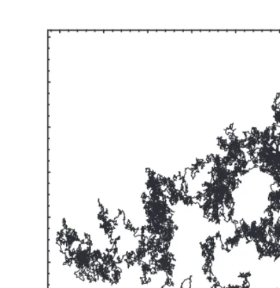
Fig. 1. – Gaussian random walk (Brownian) obtained by Monte Carlo simulation in the absence of absorption. The multiple-scattering process slows down the transport of the walker (light) in the medium with respect the homogenous scatterer-free material. This in turn induces an increase of the optical thickness of the system.
By engineering the distribution of scattering elements, control on light propagation can be achieved, with great use for photovoltaic applications. In particular, light can be slowed down in the material increasing the probability of light-matter interaction. As a consequence light can be “held” in the material longer that it would do in its homogeneous counterpart experiencing an effectively thicker material. This could be of paramount importance for photovoltaic applications, for which the reduction of material use, for economical and technical reasons, is constantly pursed.
2.2.Disordered structures and random walks. – Disordered materials can be created in a variety of ways, amongst which one of the most simple ways maybe that of grinding solids into fine powders. Alternative approaches include etching of glasses or semicon-ductors such as silicon [36] and gallium phosphide [37]. For photovoltaic application the fabrication of disorder material has to be handled with a certain care. The quality of the atomic structure has to be extremely good in order to avoid the occurrence of defect sates in the electronic band structure, ensuring a good electronic transport.
be made. Normally, the step length distribution has finite moments which unequivocally leads, due to the Central-Limit Theorem, to a normal distribution of the step size and to a Brownian-like transport (fig. 1), which in turn can be described by diffusion theory (see next section). The multiple scattering process significantly slows down the propagation of light and thus increasing the probability of absorption. The effect of absorption on light transport can be implemented easily in Monte Carlo simulations by adding a certain probabilityPa to be absorbed at each step, following the well-known Lambert-Beer’s law
Pa =e−αs, wheresis the step length andαis the absorption coefficient of the material
in which the multiple scattering occurs.
3. – Diffusion theory
In the following sections we will describe the theoretical basis that is often used to model light transport in random media. Before considering interference, our starting point is that of diffusive transport. In the diffusion approximation, the propagation of the intensity is described as a random walk with a characteristic mean free path. Only the intensity and not the electric field itself is considered, so the wave character of the light is not taken into account. Usually also the vector nature of light is disregarded. In reality, there are two polarization channels over which light is distributed in the scattering process. In practise though, often good agreement can be found between scalar diffusion theory and experimental data for light backscattered from a disordered sample when the appropriate polarization channels are considered. A typical diffusion equation for the intensityI(r, t) can be written as follows [39]:
(3.1) ∂I(r, t)
∂t =D∇
2I(r, t)− v
i
I(r, t),
whereDis the Boltzmann diffusion constant, which, in case of an exponential step-length distribution is given by D= 1
3v, withthe transport mean free path (see below), v is
the transport velocity for the light inside the medium, andi is the inelastic mean free
path. Note that a proper definition of the intensity in terms of the electric field will be given in sect.4, where we will deal with multiple scattering and include interference effects. The diffusion equation as written above is used now to introduce some basic concepts.
3.1. Important length scales for diffusive systems. – The characteristic length scales relevant for the scattering of the light, are the transport mean free path and the scattering mean free paths. The scattering mean free path is defined as the average
distance between two scattering events. For a random distribution of small particles,s
is given by
(3.2) s=
1 nσsc
withnthe density of the scattering particles andσsc their scattering cross-section. The
transport mean free pathis defined as the average distance the light travels from some arbitrary point A in the sample, before its memory of direction of propagation it had at A is lost. For isotropic scattering, is equal tos. For anisotropic scattering, and if
Anderson localization effects can be neglected, the transport mean free path is given by
(3.3) = 1
1− cosθ 1 nσsc
,
wherecosθis the average cosine of the scattering angle for one scatterer.
4. – Interference effects: transport beyond diffusion
In the diffusion approximation we are missing a fundamental aspect of light transport, namely that of interference between multiply scattered waves. To take that into account properly we have to develop a transport theory that considers the multiple scattering of the electric field instead of the intensity, in such a way that none of the phase information is lost. Starting point is the set of Maxwell’s equations for the electric and magnetic field. Green’s function theory is then used to derive perturbation expansions both for the electric field and the intensity.
Starting from Maxwell’s equations, the electric field can be shown to fulfill the time-dependent wave equation [40]:
(4.4) ∇2E(r, t) +∇E(r, t)·∇(r)
(r) −
(r) c2
0
∂2E(r, t) ∂t2 = 0.
The second term in this equation, containing the gradient of (r), is zero in regions of space where (r) is constant. We will regard a collection of particles with a constant refractive index in a surrounding medium with another constant refractive index, so(r) is constant inside and outside the particles. In that case, the second term in eq. (4.4) determines the boundary condition for the electric field at the particle boundary, and is zero elsewhere. By using a Fourier transformation with respect to time, the explicit time dependence in eq. (4.4) can be removed, and all harmonics of the resulting Fourier representation will follow the time-independent Helmholtz equation:
(4.5) ∇2E(r) + (ω/c0)2(r)E(r) = 0,
where E(r) denotes one of the field components of the electric field, inside or outside the scatterers. The same equation holds for the magnetic field components. Here(r) is the (random) place-dependent dielectric constant of the system,ω the frequency of the electric field, andc0 the vacuum speed of light. The wave equation can be written as
where V(r) is the scattering potential defined as V(r) ≡ −(ω/c0)2[(r)−1]. For a
collection of point-like scatterers with polarizability α0, in a surrounding medium with
dielectric constant 1, the scattering potential is given by
(4.7) V(r) =−α0(ω/c0)2
i
δ(r−ri),
with ri the positions of the scatterers. For a subwavelength scatterer of spherical
shape with dielectric constant 1 and radius a in vacuum, the polarizability is given
byα0=a3(1−1)/(1+ 2). Introducing the Green’s functionG0(r1,r2) as the solution
of
(4.8) ∇2G0(r1,r2) + (ω/c0)2G0(r1,r2) =−δ(r1−r2),
one can write the solution to eq. (4.6) formally as
(4.9) E(r1) =Ein(r1)−
dr2G0(r1,r2)V(r2)E(r2),
whereEin(r1) is a solution of the homogeneous wave equation obtained by takingV(r) =
0 in eq. (4.6). Ein(r1) represents the incoming coherent wave. G0(r1,r2) is also referred
to as the bare Green’s function and describes the propagation of the field in a medium without scatterers. It is given by
(4.10) G0(r1,r2) =
e−ik|r1−r2|
4π|r1−r2|
,
with k= ω/c0. By iterating the recursion relation eq. (4.9), one obtains the following
perturbation series for the electric field:
E(r1) =Ein(r1)−
dr2 G0(r1,r2)V(r2)Ein(r2)
(4.11)
+
dr2dr3 G0(r1,r2)V(r2)G0(r2,r3)V(r3)Ein(r3)
−
dr2 . . .dr4G0(r1,r2)V(r2)G0(r2,r3)V(r3)G0(r3,r4)V(r4)Ein(r4) +· · ·,
where all integrals are taken over the volume of the sample. The above expression depends onEin. To describe the propagation of the field in the medium independently
ofEin, we use the total Green’s functionG(r1,r2) which is defined as the solution of
The Green’s functionG(r1,r2) describes the field at any pointr1in the medium, due
to a source atr2. The perturbation series forG(r1,r2) is
G(r1,r2) =G0(r1,r2)−
draG0(r1,ra)V(ra)G0(ra,r2)
(4.13)
+
dradrbG0(r1,ra)V(ra)G0(ra,rb)V(rb)G0(rb,r2)− · · · .
Note thatV(r) (given by eq. (4.7)) contains the contributions from all scatterers. The first term of (4.13) describes propagation without scattering, the second term equals the sum of all single scattering contributions, the third term the sum of all double-scattering contributions, etc. To simplify the notation often Feynman-type scattering diagrams are used [38]. With such a diagrammatic notation it is easier to notice the occurrence of recurrent scattering events. These are events in which a wave is scattered by a specific scatterer, scattered by at least one other scatterer and then returns to this specific scat-terer again. For relatively weak scattering (diluted systems), recurrent scattering events can be neglected. This is the so-called independent scattering approximation in which the presence of other scatterers does not influence a single scattering. In a denser system (strong scattering) the recurrent scattering events have a more relevant contribution, but the nature of the transport remain diffusive [38].
The total Green’s functionG(r1,r2) depends on the positions of the scatterers,
re-quiring to know exactly the distribution of the scatterers to infer the transport prop-erties of the systems. A useful quantity is the averaged or “dressed” Green’s function G(r1−r2), which is obtained by averagingG(r1,r2) over the positions of the
scatter-ers. When the distribution of scatterers is truly randomized the phase of the scattered field averaged out, thus significantly simplifying the problem(1). In the self-avoiding
multiple-scattering approximation G(r1−r2) can be calculated from (4.13), by Fourier
transforming to momentum space. In momentum space the summation can be performed and after transforming back to real space one finds
(4.14) G(r1−r2)≡ G(r1,r2)=
e−iK|r1−r2|
4π|r1−r2|
,
where K = (ω/c0)2+nt is the (complex) effective k-vector for the light inside the
sample, withnthe density of scatterers.
Given the complexity of measuring fields at optical frequencies it is very useful to move from the field propagator to the intensity propagator. The intensity is defined as the energy that crosses a unit area per unit of time. It is given by the magnitude of the
cycle average of the Poynting vectorE×B, which can be written as
(4.15) I(r) = c0n
2 |E(r)|
2,
withc0 the vacuum speed of light, andn the refractive index of the medium. In terms
of the total Green’s functionG(r1,r2), the intensity is given by
(4.16) I(r)≡ c0n 2 E(r)E
∗(r) =c0n
2
dr1dr2G(r,r1)G∗(r,r2)Ein(r1)Ein∗(r2),
where G(r1,r2) is the unaveraged Green’s function. The product G G∗ describes the
intensity at any point in the system due to the product of incoming wavesEinEin∗.
In the independent scattering approximations and applying the average over different realization of disorder, transport of intensity can be described by the average propagator
G G∗. Exploiting once again the Feynman diagrams it is possible to show thatG G∗ is mostly described by two type of diagrams: the so-called “ladder” diagrams L and “most-crossed” diagramsC [41]. The ladder diagrams describe incoherent transport of the intensity while the most-crossed diagrams describe an interference phenomenon called coherent backscattering, which is explained in the next section.
4.1. Weak localization. – Maybe the most robust of interference phenomena in mul-tiple scattering is that of weak localization [42] which originates from the fundamental concept of reciprocity. In weak localization, interference leads to a net reduction of light transport similar to the weak localization phenomenon for electrons in disordered (semi)conductors and often seen as the precursor to Anderson (or strong) localization of light [43]. Weak localization of light can be observed since it manifests itself as an en-hancement of the light intensity in the exact backscattering direction. This enen-hancement is called the cone of coherent backscattering. Since the first experimental observation of coherent backscattering from colloidal suspensions [42], the phenomenon has been successfully studied in strongly scattering powders [44, 45], cold atom gases [46], semi-conductor microcavities [47], two-dimensional random systems of rods [48], randomized laser materials [49], disordered liquid crystals [50, 51], and even photonic crystals [52].
The backscattered intensity is usually described in terms of a bistatic coefficientγ(or albedo), defined as the observed scattered flux per solid angle and per unit of observed area of the sample at normalized incident flux. This coefficient is in relation with the return probability of a photon, which is, the probability that the light path in a random walk comes back at its starting point [38]. In terms of the average scattered intensity
I(r)and incident intensityI0, the bistatic coefficient can be written as
(4.17) γ= 4πr
2
A
I(r) I0
,
It is convenient to separate the total bistatic coefficientγtinto the contribution from
most-crossed diagrams γc and from ladder diagrams, with the latter further separated
into the single scattering contributionγs and multiple scattering contributionγ:
(4.18) γt=γs+γ+γc.
By making use of the propagator described in the previous paragraph, the bistatic coef-ficients can be calculated as, for single scattering:
(4.19) γs(θs) =
μs
1 +μs
1−e−Lκe(1 +μ−s1)
,
for the multiple scattering ladder diagrams (describing the diffuse background):
(4.20) γ(θs) =
3 23αsin[α(L+ 2z
0)]
Z1(1 +e−2uL) +Z2(1−e−2uL) +Z3e−L(v+u)
u[(u2−α2)2+v2(v2−2α2−2u2)]
with
Z1=u(u2−v2−α2) cos[α(L+ 2z0)] +u(v2−u2−α2) cos(αL)
(4.21)
+2uvαsin[α(L+ 2z0)] +uvα
v2−α2−3u2
u2−α2 sin(α L),
Z2=v(v2−u2−α2) cos[α(L+ 2z0)] + 2u2αsin(α L)
(4.22)
−α(u2+v2−α2) sin[α(L+ 2z0)] +u2v
u2−v2+ 3α2
u2−α2 cos(α L),
Z3= 2u(u2−v2+α2) + 2u(v2−u2+α2) cos(2z0α)−4uvαsin(2z0α),
(4.23)
and for the most-crossed diagrams (describing interference):
γc(θs) =
3e−uL 23αsinh[α(L+ 2z
0)]
1
(α2+η2+u2)2−(2αη)2
(4.24)
×−2(α2+η2+u2) cosh(2αz0) cos(Lη)−4αηsinh(2αz0) sin(Lη)
+2α u(−α
2+η2−u2) sinh(α(L+ 2z
0)) sinh(uL)
−2(α2−η2−u2) cos(Lη) + 2(α2+η2+u2) cosh(α(L+ 2z0)) cosh(uL)
+4αusinh(αL) sinh(uL)−2(−α2+η2+u2) cosh(αL) cosh(uL).
In these expressions, the angular dependence is determined by the following parameters:
η≡k(1−μs),u≡ 12κe(1+μs−1),v≡12κe(1−μ− 1
s ), andα≡ − 2
-1.5 -1.0 -0.5 0.0 0.5 1.0 1.5 0
1 2 3 4 5 6 7 8
l
+
c
Angle (rad)
0 1 2
Scaled
intensity
γ
γ
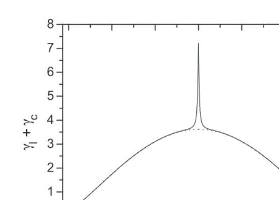
Fig. 2. – Total bistatic coefficientversusscattering angle, calculated in the diffusion approxima-tion for a non-absorbing semi-infinite disordered sample with mean free path= 5μm. Wave-lengthλ= 700 nm. Scattering angle zero corresponds to exact backscattering. The dashed line isγ, describing the diffuse background intensity. Dashed and solid lines largely overlap, except in and around exact backscattering where a narrow coherent backscattering cone is present.
As mentioned before,μs = cosθ, withθthe angle between the outgoing wave vectorks
and ˆz,Lis the sample thickness,z0= 0.7104, andκe is the extinction coefficient given
byκe =−s1+−i 1. In the limitL→ ∞ (i.e.for a semi-infinite slab), the expression for
γc reduces to
(4.25) γc(θs) =
3 23αu
α+u(1−e−2αz0)
(u+α)2+η2 .
The physical interpretation ofγandγcis the following. γdescribes the (incoherent)
backscattered intensity due to diffusion without interference. Its angular dependence is weak (see dashed line fig. 2): it decreases slowly at larger angles. This angular depen-dence is due to the fact that under larger outgoing angles, the light travels through a larger part of the sample, having a larger chance to be scattered or absorbed. The inten-sity described byγc originates from interference between reciprocal waves(2). Because a
random dielectric system obeys reciprocity, any partial wave that propagates over some distance through the sample and then leaves the illuminated area in the backscattering
(2) Optical measurements on linear physical systems obey the general principal of reciprocity,
direction will have a counterpropagating counterpart that follows the same path in the opposite direction. These counterpropagating partial waves have travelled over the same distance in the sample and interfere therefore constructively in the backscattering direc-tion. This is what is described by the most-crossed diagrams. The angular dependence of γc is strong: it decays rapidly moving away from the exact backscattering direction
(see solid line fig. 2). Away from exact backscattering, a phase difference develops be-tween the counterpropagating waves that depends on the relative orientation of the points where the waves leave the sample. For the ensemble of light paths, the relative phases will therefore gradually randomize. After averaging over all light paths, this leads to the cone of enhanced backscattering described byγc [38].
Given the relation between the bistatic coefficient and the return probability, we immediately infer (fig. 2) that the probability of return to the origin is twice as large as what one would expect from diffusion theory, due to the interference effect. As the scattering strength increases, the cone becomes larger, and thus the probability that the light paths bends back increases with respect to diffusion.
4.2.Strong localization. – The most surprising of interference phenomena in random systems is that of Anderson localization, which was originally discovered for electron transport. In Anderson localization of light, diffusion comes to a halt due to interfer-ence(3). When the scattering strength of a material is increased (and hence further
decreased), a phase transition into an Anderson localized state is expected to occur at k≤1, withkthe wave vector of the light [32, 54]. Fork >1 the transport is diffusive, which is the case in most of the available disordered dielectric materials.
Ideally such reduction of transport could be exploited for photovoltaic applications. Strong localization of light in 3D random systems requires, however, very strong scatter-ing and, although some experimental evidence of its existence has been shown [32], no direct observation of this phenomena for 3D systems has been reported so far. Neverthe-less, in order to obtain an significant enhancement of the absorption, it should be enough to work at the transition threshold, the so-called mobility edge. It has been predicted, but yet not experimentally proven, that for strong enough scattering strength, close to the localized regime, transport is slow down so much that light absorption significantly increases [55].
The phenomenon can be studied also in lower-dimensional systems like random di-electric multi-layers (1D) [56-58], see fig. 3a, or random holes distribution in thin films (2D) [25], see fig. 4a. One and two-dimensional optical systems have the advantage that, for large enough samples, localization always sets in (fig. 3b and 4b). That is, there is no phase transition as described above for 3D systems and transport is dominated by localized modes independently of the amount of disorder.
To what extent Anderson localization can help for absorption enhancement is still
A A A A A A
B B B B B
Random stack
a)
b)
Fig. 3. – a) One-dimensional disordered photonic systems. By stacking two types of layers (A and B have e different refractive index), one can obtain a random one-dimensional structure. b) Energy distribution in a random system. Anderson localized modes occur as resonances randomly distributed along the system and at random frequencies. Localized modes can also couple into de-localized or necklace modes, that extend over the whole structure.
under investigation. Three-dimensional systems in which light unequivocally localized are still to be discovered and thus possible applications can only be hypothetical. Much more promising are 2D structures [22], for which disorder photonic media can fabricated with techniques compatible with state-of-the-art solar cells fabrication methods.
a)
b)
a)
b)
Fig. 5. – a) Extinction SCS, scattering SCS and absorption SCS of aluminum nanoparticles of 50 nm and 70 nm of diameter. b) Measured and calculated absorption enhancement of a suspension of such an aluminum nanoparticle in dye.
5. – Alternative photonic strategies
So far we have been dealing with disordered system made out of dielectric materials. However, in the last decade an increasing interest for metal-dielectric nanostructures to exploit for photovoltaic applications is developing [59]. The advantage of using metallic scattering elements is primarily due to complex permittivity of the constituent materials (e.g., gold, silver, aluminum, etc.) which has a two-fold consequence on the optical response of the nano-object: i) the optical properties are often resonant, allowing to select a certain spectral range, and ii) a huge field enhancement close to the object surface can occur, increasing tremendously the light matter interaction in the vicinity of the object. Both effects are due to a coupled state between the electrons bound to the metal and the impinging electromagnetic wave, the so-calledplasmon polariton [60]. Also in this case the photonic structure can be periodic (e.g., nanostructured backreflectors [61] or arrays of nanoparticles [62]), or disordered (e.g., disordered arrays [63] or suspensions of metallic nanoparticles [64]). In fig. 5a the calculated extinction, scattering and absorption cross-sections (SCS) for aluminum nanoparticles of diameter 50 nm and 70 nm is shown [64]. The choice of the radius and material employed has been made to obtain a resonant effect of the scattering properties to harvest the UV region of the solar radiation. In this way a suspension of these particles in an absorbing medium increases the optical path of the UV radiation, as shown by the measured and calculated absorption enhancement in fig. 5b, leaving almost unperturbed the propagation of light at different frequencies.
6. – Conclusions
approaches used with this intent [17] and still its application in the photovoltaic field is vastly studied. Due to the optical “robustness” it can provide, the broadband re-sponse and the possibility to grow cheap structures, it is interesting to study disordered architectures for future implementation in new generation of solar cells.
∗ ∗ ∗
This work was financially supported by the European community via the NoE on Nanophotonics for Energy.
REFERENCES
[1] Schaller R. D., Sykora M., Pietryga J. M.andKlimov V. I.,Nano Lett.,6(2006) 424.
[2] Zahler J. M.et al.,App. Phys. Lett.,91(2007) 012108. [3] Granqvist C. G.,Sol. Energ. Mater. Sol. C,91(2007) 1529. [4] Brown G.andWu J.,Laser Photon. Rev.,3(2009) 394. [5] Chen H.et al.,Nat. Photon.,3(2009) 649.
[6] Krebs F. C.,Sol. Energ. Mater. Solar C,93(2009) 394. [7] Andreev V. M.et al.,Sol. Energ. Mater. Sol. C,84(2004) 17.
[8] Spinelli P., Verschuuren M.andPolman A.,Nat. Commun.,3(2012) 692. [9] Han S. E.andChen G.,Nano Lett.,10(2010) 1012.
[10] Atwater H. A.andPolman A.,Nat. Mater.,9(2010) 205. [11] Ferry V. E.et al.,Nano Lett.,11(2011) 4239.
[12] Meng X.et al.,Sol. Energ. Mater. Solar C,95,Suppl. 1(2011) S32. [13] Mallick S. B.et al.,App. Phys. Lett.,100(2012) 053113.
[14] Yu Z., Raman A.andFan S.,Proc. Natl. Acad. Sci. U.S.A.,107(2010) 17491. [15] Callahan D. M., Munday J. N.andAtwater H. A.,Nano Lett.,12(2012) 214. [16] Bozzola A., Liscidini M.andAndreani L. C.,Opt. Express,20(2012) A224. [17] Yablonovitch E.,J. Opt. Soc. Am. A,72(1982) 899.
[18] Yu Z., Raman A.andFan S.,Phys. Rev. Lett.,109(2012) 173901.
[19] Rockstuhl C., Fahr S., Bittkau K., Beckers T., Carius R., Haug F.-J.,
S¨oderstr¨om T., Ballif C.andLederer F.,Opt. Express,18(2010) 335.
[20] Martins E. R., Li J., Liu Y., Zhou J. and Krauss T. F., Phys. Rev. B,86 (2012) 041404.
[21] Oskooi A., Favuzzi P. A., Tanaka Y., Shigeta H., Kawakami Y.andNoda S.,App. Phys. Lett.,100(2012) 181110.
[22] Vynck K., Burresi M., Riboli F.andWiersma D. S.,Nat. Mater.(2012).
[23] Sigalas M. M., Soukoulis C. M., Chan C.-T.andTurner D.,Phys. Rev. B,53(1996) 8340.
[24] Vanneste C.andSebbah P.,Phys. Rev. A,79(2009) 041802. [25] Riboli F.et al.,Opt. Lett.,36(2011) 127.
[26] Yablonovitch E.,Phys. Rev. Lett.,58(1987) 2059;John S.,Phys. Rev. Lett.,58(1987) 2486.
[27] Soukoulis C. M. (Editor), Photonic Bandgap Materials (Kluwer, Dordrecht) 1996; Joannopoulos J. D., Meade R. D. and Winn J. N., Photonic Crystals (Princeton University Press, Princeton, NJ) 1995.
[29] Kuga Y. andIshimaru A.,J. Opt. Soc. Am. A,8(1984) 831;van Albada M. P.and Lagendijk A.,Phys. Rev. Lett.,55(1985) 2692;Wolf P. E.andMaret G.,Phys. Rev. Lett.,55(1985) 2696.
[30] van Tiggelen B. A., Phys. Rev. Lett., 75 (1995) 422; Rikken G. L. J. A. and van Tiggelen B. A.,Nature,381(1996) 54.
[31] Sparenberg A., Rikken G. L. J. A. andvan Tiggelen B. A., Phys. Rev. Lett., 79 (1997) 757.
[32] John S.,Phys. Rev. Lett.,53(1984) 2169;Anderson P. W.,Philos. Mag. B,52(1985) 505; Dalichaouch R. et al., Nature, 354 (1991) 53; Wiersma D. S. et al., Nature (London), 390(1997) 671; Chabanov A. A. and Genack A. Z., Phys. Rev. Lett., 87 (2001) 153901; St¨orzer M., Gross P., Aegerter C. M. and Maret G., Phys. Rev. Lett.,96(2006) 063904;van der Beek T., Barthelemy P., Johnson P. M., Wiersma D. S.andLagendijk A.,Phys. Rev. B,85(2012) 115401.
[33] Sapienza R., Costantino P., Wiersma D. S., Ghulinyan M., Oton C.and Pavesi L.,Phys. Rev. Lett.,91(2003) 263902.
[34] Ghulinyan M., Oton C., Gaburro Z., Pavesi L., Toninelli C.andWiersma D. S., Phys. Rev. Lett.,94(2005) 127401.
[35] Scheffold F.andMaret G.,Phys. Rev. Lett.,81(1998) 5800. [36] Bisi O., Ossicini S. andPavesi L.,Surf. Sci. Rep.,38(2000) 1.
[37] Schuurmans F. J., Vanmaekelbergh D., van de Lagemaat J. and Lagendijk A., Science,284(1999) 141.
[38] Akkermans E. and Montambaux G., Mesoscopic Physics of Electrons and Photons (Cambridge University Press) 2007.
[39] Martelli F., Contini D., Taddeucci A. andZaccanti G.,Appl. Optics, 36(1997) 4600.
[40] Jackson J. D.,Classical Electrodynamics (Wiley, New York) 1975. [41] Vollhardt D.andW¨olfle P.,Phys. Rev. B,22(1980) 4666.
[42] Kuga Y. and Ishimaru A., J. Opt. Soc. Am. A, 8 (1984) 831; Albada M. V. and Lagendijk A., Phys. Rev. Lett., 55(1985) 2692; Wolf P. andMaret G., Phys. Rev. Lett.,55(1985) 2696.
[43] John S.,Phys. Rev. Lett.,53(1984) 2169;Anderson P. W.,Philos. Mag. B,52(1985) 505.
[44] Kaveh M.et al.,Phys. Rev. Lett.,57(1986) 2049. [45] Wiersma D. S.et al.,Phys. Rev. Lett.,74(1995) 4193.
[46] Labeyrie G. et al., Phys. Rev. Lett.,83 (1999) 5266;Labeyrie G. et al.,J. Opt. B -Quantum and Semiclassical Optics,2 (2000) 672; Bidel Y. et al., Phys. Rev. Lett., 88 (2002) 203902.
[47] Gurioli M.et al.,Phys. Rev. Lett.,94(2005) 183901. [48] Freund I.et al.,Phys. Rev. Lett.,61(1988) 1214.
[49] Wiersma D. S., van Albada M. P. and Lagendijk A., Phys. Rev. Lett., 75 (1995) 1739.
[50] Vlasov D. V. et al., Pisma Zh. Eksp. Teor. Fiz.,48(1988) 86 (JETP Lett.,48(1988) 91).
[51] Kuzmin L. V., Romanov V. P.andZubkov L. A.,Phys. Rev. E,54(1996) 6798. [52] Koenderink A. F. et al., Phys. Lett. A, 268(2000) 104; Huang J. et al.,Phys. Rev.
Lett.,86(2001) 4815.
[53] van Tiggelen B. A., Lagendijk A. andWiersma D. S.,Phys. Rev. Lett.,84(2000) 4333.
[55] John S.,Phys. Rev. Lett.,53(1987) 2169.
[56] Bliokh K. Y., Bliokh Y. P., Freilikher V., Genack A. Z., Hu B.andSebbah P., Phys. Rev. Lett.,97(2006) 243904.
[57] Bertolotti J., Galli M., Sapienza R., Ghulinyan M., Gottardo S., Andreani L. C., Pavesi L.andWiersma D. S.,Phys. Rev. E,74(2006) 035602.
[58] Bertolotti J., Gottardo S., Wiersma D. S., Ghulinyan M. andPavesi L., Phys. Rev. Lett.,94(2005) 113903.
[59] Atwater H.andPolamn A.,Nat. Mater,9(2010) 205.
[60] Pitarke J. M., Silkin V. M., Chulkov E. V.andEchenique P. M.,Rep. Prog. Phys.,
70(2007) 1.
[61] Fahr S., Rockstuhl C. andLederer F.,App. Phys. Lett.,95(2009) 121105. [62] Schaadt D. M., Feng B. andYu E. T.,App. Phys. Lett.,86(2005) 063106. [63] Nishijima Y., Rosa L.andJuodkazis S.,Opt. Express,20(2012) 11466.