Real-time ﬂood forecasting coupling different postprocessing techniques of precipitation forecast ensembles with a distributed hydrological model. The case study of may 2008 ﬂood in western Piemonte, Italy

(1)

Nat. Hazards Earth Syst. Sci., 13, 211–220, 2013 www.nat-hazards-earth-syst-sci.net/13/211/2013/ doi:10.5194/nhess-13-211-2013

EGU Journal Logos (RGB)

Advances in

Geosciences

Open Access

Natural Hazards

and Earth System

Sciences

Open Access

Annales

Geophysicae

Open Access

Nonlinear Processes

in Geophysics

Open Access

Atmospheric

Chemistry

and Physics

Open Access

Atmospheric

Chemistry

and Physics

Open Access Discussions

Atmospheric

Measurement

Techniques

Open Access

Atmospheric

Measurement

Techniques

Biogeosciences

Open Access Open Access

Biogeosciences

Discussions

Climate

of the Past

Climate

of the Past

Discussions

Earth System

Dynamics

Earth System

Dynamics

Discussions

Geoscientific

Instrumentation

Methods and

Data Systems

Open Access

_{Geoscientific}

Instrumentation

Methods and

Data Systems

Geoscientific

Model Development

Geoscientific

Model Development

Discussions

Hydrology and

Earth System

Sciences

Open Access

Hydrology and

Earth System

Sciences

Ocean Science

Discussions

Solid Earth

Discussions

The Cryosphere

Natural Hazards

and Earth System

Sciences

Open Access

Discussions

Real-time flood forecasting coupling different postprocessing

techniques of precipitation forecast ensembles with a distributed

hydrological model. The case study of may 2008 flood in western

Piemonte, Italy

D. Cane, S. Ghigo, D. Rabuffetti, and M. Milelli

Regional Agency for Environmental Protection – Arpa Piemonte, Torino, Italy

Correspondence to: D. Cane ([email protected])

Received: 10 January 2012 – Published in Nat. Hazards Earth Syst. Sci. Discuss.: – Revised: 18 May 2012 – Accepted: 19 June 2012 – Published: 5 February 2013

Abstract. In this work, we compare the performance of an

hydrological model when driven by probabilistic rain fore-cast derived from two different post-processing techniques. The region of interest is Piemonte, northwestern Italy, a com-plex orography area close to the Mediterranean Sea where the forecast are often a challenge for weather models. The May 2008 flood is here used as a case study, and the very dense weather station network allows us for a very good de-scription of the event and initialization of the hydrological model. The ensemble probabilistic forecasts of the rainfall fields are obtained with the Bayesian model averaging, with the classical poor man ensemble approach and with a new technique, the Multimodel SuperEnsemble Dressing. In this case study, the meteo-hydrological chain initialized with the Multimodel SuperEnsemble Dressing is able to provide more valuable discharge ranges with respect to the one initialized with Bayesian model averaging multi-model.

1 Introduction

High resolution spatiotemporal rainfall intensity forecasts are the main input into rainfall-runoff models for flood forecast, debris-flow and landslide triggering. For supporting deci-sion makers in order to assure a good prevention act regard-ing overflows or floods, environmental agencies implement deterministic models returning hydro-meteorological predic-tions on a regular grid with a certain spatial resolution. These numeric models approximate mathematically the underlying

physical and chemical dynamics through complex non linear differential equations. However, very few operational hydro-meteorological chains provide an estimate of the uncertain-ties of the results: rainfall forecasts, due to its complex na-ture, are heavily affected by many sources of uncertainty. A very exhaustive review on the different sources of uncertain-ties in the meteo-hydrological chain can be found in Cloke and Pappenberger (2009): they can arise from observations, from NWP model initial conditions, from NWP model pa-rameterizations, or from the hydrological model initialization and design.

Forecast uncertainty due to the partial knowledge of the initial conditions is usually tackled by ensemble predic-tions systems (EPS), where a set of forecast runs are per-formed from perturbed initial conditions: for instance, Zappa et al. (2010) explore the propagation of uncertainty from ob-serving systems and NWP into hydrological models, based on global model EPS and limited area model EPS.

A second class of uncertainties arises from the choices in model implementation (domain size, resolution, hydro-static/non hydrostatic approach, physical parameterizations, etc.: an interesting experiment on how changes on a single model implementation can produce quite different rainfall extimations can be found in Stensrud et al., 2000), and can be targeted with multi-physics systems, like in Amengual et al. (2008), where different parametrizations of a single model are used to produce an ensemble of rainfall extimations to run an hydrological model, or from multi-model EPS systems, as proposed by Cloke and Pappenberger (2009).

(2)

A further possibility is the use of already available op-erational NWP models to obtain a multi-model set where the final value may derive from an average, as in Raftery et al. (2005), or from a selection procedure, as in Roulston and Smith (2003), where the Best Member Dressing method is proposed. Probabilistic forecasting is a relatively new ap-proach which may properly account for all sources of uncer-tainty. Recently, Sloughter et al. (2007) have extended the Bayesian model averaging (BMA) framework of Raftery et al. (2005) in order to derive probabilistic precipitation fore-cast via a mixture distribution. BMA belongs to the method-ologies of ensemble forecasting, that considers not only a single deterministic forecast but joint forecasts coming from different models and initial conditions.

The Multimodel SuperEnsemble technique is another powerful statistical method for a better estimation of weather forecast parameters with weights calculated in a training pe-riod, originally proposed by Krishnamurti et al. (1999). Cane and Milelli (2006) have already applied it in Piemonte re-gion (north-western Italy), a complex orographic area, to provide a more accurate forecast of several weather parame-ters, including precipitation (Cane and Milelli, 2010a). Fur-thermore, Cane and Milelli (2010b) proposed a probabilistic quantitative precipitation forecasting (QPF) evaluation with the use of a new Multimodel SuperEnsemble Dressing tech-nique. This new approach, providing an estimation of the probability density function (PDF) of precipitation, widens our knowledge of the precipitation field characteristics, is a support for operational weather forecast and can also be used as input for the hydrological forecast chain, propagat-ing the QPF uncertainty to the evaluation of its effects on the territory. The probabilistic scores of this technique are proven better than the Multimodel probabilistic technique originally proposed by Stefanova et al. (2002) (Cane and Milelli, 2010b).

In this paper, our purpose is to compare the performance of hydrological real-time forecasts when rainfall fields are re-alized as ”ensemble prediction” which consider jointly pre-dicted rainfall fields provided by several numerical models or different initial status in the same model. In particular, we focus on three different post-processing techniques of deter-ministic precipitation forecasts. Firstly, following Sloughter et al. (2007), Bayesian model averaging (BMA) will be taken into account using asymmetric distributions, which char-acterized rainfall data. Therefore, mixture models are em-ployed where first the probability of rain is modelled and then, conditionally on the former event (it does not rain or it rains), a continuous skewed distribution is used for rain-fall. Secondly Multimodel SuperEnsemble Dressing (MSD) is applied on the same data, providing adjusted probability density functions of the rainfall fields. As a benchmark, we explore the poor man ensemble (PME) technique, that con-sists in a merely arithmetic mean of deterministic data in-stead. Therefore, this methodology does not take into account uncertainty. Once forecast rainfall amounts are obtained, they

are used as input for the hydrological water-balance model FEST-WB, implemented by the environmental agency Arpa Piemonte, in order to assess flood formation and propagation in hydrographical network.

We applied this simulation exercise to the case study of May 2008 flood in western Piemonte, Italy. Far from being exhaustive for a sound statistical validation of the conclusion, the results obtained shows the feasibility of a real time appli-cation of the hydrometeorological chain proposed and offer a starting point for further investigation.

The paper is organized as follows. The three different post-processing techniques and the hydrological model are explained in Sect. 2. Section 3 outlines the detail of the hydro-meteorological coupling and of the application, while in Sect. 4, we provide a description of the analysed catch-ments and event. In Sect. 5, we illustrate the results of the hy-drological model using as input rainfall amounts forecasted by means of the three different post-processing techniques concerning the case study of May 2008 flood. Finally, Sect. 6 includes discussion on findings.

2 Model description

The forecasts of rainfall fields are usually performed by means of deterministic models, characterized however by two main sources of uncertainty: errors connected with start-ing conditions and model errors. The standard “ensemble forecasting” method requires many runs of a single model with perturbed starting values, trying to cover all the spread of the initial conditions and tackle the error coming from the first source of uncertainty. The Multimodel approach tries to solve the uncertainty coming from the incomplete represen-tation of reality by the models. In this paper we explore three different multi-model post-processing techniques of deter-ministic precipitation forecasts in order to estimate the fore-cast rainfall probabilities: Bayesian model averaging, Multi-model SuperEnsemble Dressing and poor man ensemble: we review here some theory and set the notation for each pro-cedure. Moreover, since we want to evaluate flood formation and propagation using as input these three different forecasts, here we give some essential information about the hydrolog-ical water-balance model FEST-WB.

2.1 Bayesian model averaging

Bayesian model averaging is a statistical method for com-bining forecasts from different models conditioning, not on a single “best” model, but on the entire ensemble of statistical models first considered. Despite the basic paradigm for this technique was introduced by Leamer (1978), the approach was basically ignored until the late 1990s and 2000s when there was an enormous amount of literature on the use of BMA (e.g. Clyde, 1999, Hoeting et al., 1999, Raftery et al., 2005, and Sloughter et al., 2007).

(3)

LetF1,. . . ,FK be a set of K deterministic forecasts un-der consiun-deration: the idea is that among these ensemble members, there is a model that comes near observations more than the others and BMA measures the uncertainty about the “best” member. Asy is the quantity to be forecasted on the basis of training observationsyT and usingKdeterministic models, the forecast PDFp(y)is given by

p(y)= K X

k=1

p(y/Fk)p(Fk/yT), (1)

where p(y/Fk) is the forecast PDF only based on model Fk, whilep(Fk/yT)is the posterior probability of modelFk given the training datayT; this term tells us how modelFk fitsyT. Since the sum of all the posterior model probabilities is equal to one, they can be viewed as weights. Moreover, to quantify the uncertainty about the best member in the ensem-ble, the forecastFkis associated with a conditional PDF, that is the conditional PDF ofygiven thatFkis the “best” ensem-ble member (gk(y/Fk)). Then, the BMA predictive model is

p(y/Fk)= K X

k=1

wkgk(y/Fk), (2)

wherewk is the posterior probability of forecastFk, that is the best one and takes into accountFk performance during the training period. Beingwk’s probabilities, they add up to 1.

The normal distribution is not appropriate to fit the precip-itation conditional PDF because rain height is zero in a large number of time points; where it is not zero, the distributions are very skewed. Thus a mixture model for the predictive PDF, as

p(y/Fk)= K X

k=1

wkP (y=0/Fk)

I[y=_0]+P (y >0/Fk)gk(y/Fk)I[y >0], (3) is implemented.P (y >0/Fk)is the probability of nonzero precipitation given the forecastFk, ifFk is the best ensem-ble member for that time point. The PDF of precipitation amount (given that it is not zero) is fitted through a gamma distribution.

2.2 Poor man ensemble

Since the 1970s the advantage of ensemble forecasting over single-run deterministic forecasting was shown by Leith (1974), proving how ensemble averaging can reduce the forecast error variance for an initial sample of normal, random initial analyses. In recent years the ensemble average has repeatedly been shown to give a more accurate forecast than a single realization of the forecast model (e.g. Du et al., 1997, Ziehmann, 2000 and Ebert, 2001). The ensemble aver-aging or poor man ensemble procedure provides a value for

each time point, that is obtained through the arithmetic mean of ensemble members at each point. Thus,

y= 1 K

K X

k=1

Fk, (4)

wherey is the forecasted rain height andFk, k=1,. . . , K, the used deterministic model forecasts, as above mentioned. This technique does not take into account any information given by observations and uncertainty given by different sources.

2.3 Multimodel SuperEnsemble Dressing

The Multimodel SuperEnsemble Dressing is a new tech-nique, firstly proposed in Cane and Milelli (2010b). They evaluated probabilistic forecasts of average and maximum precipitation on Piemonte warning areas, here it is extended to station values.

In the training period the observed precipitation probabil-ity densprobabil-ity function (PDF), conditioned to the forecasts of each model, is calculated: for a large set of model forecast values, we evaluate the observed precipitation that occurred in reality and we built a set of empirical PDFs from the fre-quency of occurrence of observed rainfall over a wide spec-trum of possible values. The moments (mean value and vari-ance) of the so-obtained QPFs correlate strongly (r2>0.98), as expected, and allow for a interpolation/extrapolation of the empirical relationship among them. This fitted relation is used to evaluate numerically the λ and k parameters of a Weibull (Weibull, 1951) distribution, fitting the observed QPFs in a very suitable way.

The calculated QPFs of the given model deterministic forecasts are used to weight them with weights obtained as the inverse of the continuous rank probability score (CRPS) evaluated in the training period for each model.

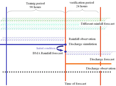
A full PDF for the Multimodel dressed (super) Ensemble is thus obtained. A scheme of the procedure is depicted in Fig. 1.

A careful evaluation of the Multimodel performances ver-sus the observations in terms of Brier skill score, roc area skill score, ignorance skill score was performed, showing a significant improvement of this technique versus the poor man ensemble probabilistic forecasts (please refer to Cane and Milelli, 2010b for a more detailed description).

2.4 Flash – flood event spatially based distributed rainfall – runoff transformation – including water balance (FEST-WB)

(4)

Fig. 1. Scheme of the Multimodel SuperEnsemble Dressing tech-nique.

Fig. 2. Scheme of the hydro-meteorological coupling.

water fluxes are calculated. The model needs spatially dis-tributed meteorological forcing. The observed data at ground stations are interpolated to a regular grid using the inverse distance weighting technique.

The snow model includes the snow melt and the snow ac-cumulation dynamics. The partitioning of total precipitation, in liquid and solid phases is a function of air temperature. The snow melt simulation is based on the classical degree day model.

Soil moisture evolution for the generic cell at positioni,j, is described by the water balance equation:

∂θi,j ∂t =

1 Zi,j

Pi,j−Ri,j−Di,j−ETi,j, (5)

whereP is the liquid precipitation rate,Ris runoff flux,Dis drainage flux, ET is evapotranspiration rate andZis the soil depth.

Fig. 3. Analysis of the geopotential height at 500 hPa (dam) from ECMWF on 29 May at 12:00 UTC.

Runoff is computed according to a modified SCS-CN method extended for continuous simulation (Ravazzani et al., 2007) where the potential maximum retention,S, is updated at the beginning of a storm as a linear function of the degree of saturation,ε.

S=S1·(1−ε) (6) whereS1 is the maximum value of S when the soil is dry (AMC 1).

The actual evapotranspiration, ET, is computed as a frac-tion of the potential rate tuned by the beta funcfrac-tion that, in turn, depends on soil moisture content (Montaldo et al., 2003). Potential evapotranspiration is computed with a radiation-based equation (Priestley and Taylor, 1972).

The surface and subsurface flow routing is based on the Muskingum-Cunge method in its non-linear form with the time variable celerity (Montaldo et al., 2007).

3 Hydro-meteorology coupling

The information we are going to use in order to estimate rainfall heights consists of output of observed data gath-ered from 278 automatic weather stations of the monitor-ing network in Piemonte and the surroundmonitor-ing area run by ARPA Piemonte, and two different deterministic models: the ECMWF IFS model and three versions of the COSMO limited area model (COSMO-I7, COSMO-7, COSMO-EU: please see www.cosmo-model.org for more details about the Consortium and the model). The rain gauge network is dense enough to achieve a very good description of the study area (Fig. 4). The resolution of the IFS model grid was approx-imately 40 km (0.25◦) , while the COSMO models had a resolution around 7 km (0.0625◦). The global model has a resolution quite coarse for the considered basins (Chisone: 560 km2, Dora Riparia: 740 km2, Pellice: 1015 km2), while the limited area models are representative enough, but the use

(5)

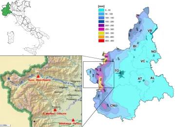
Fig. 4. On the right: total rainfall from 27 to 30 May 2008. On the left a detail of the studied area (map obtained with CAE Maps & View©) with the Dora Riparia, Chisone and Pellice catchments, where the most important damages occurred. Triangles show the hydrometers closing the three catchments, circles represent the rain gauges.

of both a global model and limited area model gave quite suc-cessful results when combined in multi-models in Piemonte region (Cane and Milelli, 2010a).

The models are interpolated bi-linearly on station loca-tions to allow a fair comparison with observaloca-tions and to provide a model input at the same nominal resolution of the observed fields. The interpolation can of course introduce systematic errors, nevertheless the interpolated model data comparison with the observations for the whole training pe-riod of both BMA and MSD, favour the bias correction; bi-ases can still influence the PME results. In this paper we take into account the 3-hourly cumulated precipitation concern-ing the flood event that from 27 to 30 May 2008 affected Piemonte region.

Concerning BMA, we choose to employ a training period of 24 data, or rather 3 days, performing model runs at dif-ferent lags (1, 2, 3 and 4 steps) in order to fit the model and obtain a forecast for the following 12 h.

Both BMA and MSD provide the predictive probability density function for each forecast time point. Since it is not possible to implement a hydrological model for each rain quantile because it is too time-consuming, we choose as in-put the 50th and 90th quantiles: thus we can observe if the flood trend is more or less well-included inside the range ob-tained using these quantiles as rainfall input.

1

Figure 5: Observed and FEST simulated discharge for May 29-30, 2008 in San Martino Chisone station 2

starting from BMA forecast of 50th and 90th quantiles and lags of 1, 2, 3 and 4 time points. 3

4

Figure 6: Observed and FEST simulated discharge for May 29-30, 2008 in San Martino Chisone station 5

Fig. 5. Observed and FEST simulated discharge for 29– 30 May 2008 in San Martino Chisone station starting from BMA forecast of 50th and 90th quantiles and lags of 1, 2, 3 and 4 time points.

(6)

18

Observed and FEST simulated discharge for May 29-30, 2008 in San Martino Chisone station

2

starting from BMA forecast of 50th and 90th quantiles and lags of 1, 2, 3 and 4 time points.

3

4

Figure 6: Observed and FEST simulated discharge for May 29-30, 2008 in San Martino Chisone station

5

starting from MSD forecast of 50th and 90th quantiles.

6 Fig. 6. Observed and FEST simulated discharge for 29– 30 May 2008 in San Martino Chisone station starting from MSD forecast of 50th and 90th quantiles.

19 1

Figure 7: Observed and FEST simulated discharge for May 29-30, 2008 in San Martino Chisone station

2

starting from PME forecast.

3

4

Figure 8: Observed and FEST simulated discharge for May 29-30, 2008 in Susa Dora Riparia station

5

6

Fig. 7. Observed and FEST simulated discharge for 29– 30 May 2008 in San Martino Chisone station starting from PME forecast.

Moreover, using the PME technique, an arithmetic mean of the five deterministic rainfall fields is done as introduced above, the forecast is characterized by one deterministic value for each time horizon.

The coupling of the quantitative rainfall forecast with the hydrological model is addressed in a “real time” setting. The hydrological model is run every three hours updating the rainfall observations series up to the time of forecast and the rainfall forecast. The grid resolution used in this work is 1 km, the same used for the whole Po catchment operational flood forecast. This resolution is a good compromise between hydrological model needs and rainfall field estimation from the gauge network while it is of course a challenge for de-terministic quantitative rainfall forecast. The post-processing techniques here proposed are tested in the general framework to overcome this dichotomy in characteristic scales in meteo-rology and mountain catchment hydmeteo-rology. A scheme of the hydro-meteorological coupling can be found in Fig. 2.

19

3

4

Figure 8: Observed and FEST simulated discharge for May 29-30, 2008 in Susa Dora Riparia station

5

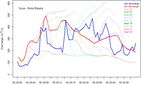
6 Fig. 8. Observed and FEST simulated discharge for 29– 30 May 2008 in Susa Dora Riparia station starting from BMA fore-cast of 50th and 90th quantiles and lags of 1, 2, 3 and 4 time points.

20 1

2

Figure 9: Observed and FEST simulated discharge for May 29-30, 2008 in Susa Dora Riparia station 3

starting from MSD forecast of 50th and 90th quantiles. 4

5

6

Fig. 9. Observed and FEST simulated discharge for 29– 30 May 2008 in Susa Dora Riparia station starting from MSD fore-cast of 50th and 90th quantiles.

4 Description of the catchments and the event

From 27 to 30 May 2008, the Piemonte region (North-Western Italy) was affected by heavy precipitation that trig-gered a number of effects on the slopes and along the rivers. An Atlantic through was stationary on the west Mediter-ranean and produced warm and humid southerly fluxes on Piemonte causing precipitation from 27 May in the northern part of the region. On 29 May, the minimum slowly started moving eastward onto the Ligurian sea (Fig. 3). This pro-duced a cold air advection in the upper levels, making the humid atmosphere unstable. Precipitation intensity increased in the north with peaks in Anza and Orco valleys in the early morning. The successive rotation of the winds to the east, and their intensification, enhanced the orographic effect on the precipitation over the Western Alps, which were hit hard-est from the late morning to the late afternoon, from Susa to Pellice and finally to Grana valleys.

The freezing level stayed above 3000 m a.s.l during the whole period so that the snow accumulation was negligible

(7)

D. Cane et al.: Real-time flood forecasting coupling different postprocessing techniques of precipitation forecast 217

20 2

Figure 9: Observed and FEST simulated discharge for May 29-30, 2008 in Susa Dora Riparia station 3

starting from MSD forecast of 50th and 90th_quantiles. 4

5

6

Fig. 10. Observed and FEST simulated discharge for 29– 30 May 2008 in Susa Dora Riparia station starting from PME fore-cast.

21 Figure 10: Observed and FEST simulated discharge for May 29-30, 2008 in Susa Dora Riparia station 1

starting from PME forecast. 2

3

Figure 11: Observed and FEST simulated discharge for May 29-30, 2008 in Pellice Villafranca station 4

6

Fig. 11. Observed and FEST simulated discharge for 29– 30 May 2008 in Pellice Villafranca station starting from BMA fore-cast of 50th and 90th quantiles and lags of 1, 2, 3 and 4 time points.

while the melting of the antecedent snow cover below that el-evation strongly contributed to amplify the total precipitation volume. Most of the alpine rain gauges records were over 200 mm, and, in the hardest hit areas, rainfall height reached 337 mm and 425 mm during the entire event respectively in the Pellice and Germanasca valleys (Fig. 4) with maximum of 24 h accumulation over 200 mm corresponding to a return period of 20–50 yr.

Very important floods were observed along the main rivers from Dora Riparia to Grana in the western Alps and pro-duced serious damages to streets and bridges. Flood waves propagated into the Po river which reached high danger lev-els upstream Torino. Shallow landslides occurred in many areas in the upstream parts of the valleys. In the northern part: Orco and Anza. In the western part: Pellice, Germasca, Po and Grana. For more details please refer to the report by Arpa Piemonte (2008).

21 starting from PME forecast.

2

3

Figure 11: Observed and FEST simulated discharge for May 29-30, 2008 in Pellice Villafranca station 4

6

Fig. 12. Observed and FEST simulated discharge for 29–30 May 2008 in Villafranca Pellice station starting from MSD forecast of 50th and 90th quantiles.

22 Figure 12: Observed and FEST simulated discharge for May 29-30, 2008 in Villafranca Pellice station

1

starting from MSD forecast of 50th and 90th quantiles.

2

3

Figure 13: Observed and FEST simulated discharge for May 29-30, 2008 in Villafranca Pellice station

4

5 Fig. 13. Observed and FEST simulated discharge for 29– 30 May 2008 in Villafranca Pellice station starting from PME fore-cast.

5 Results

Figures 5–13 represent simulated discharge trends for differ-ent forecasted time points in three station mainly stricken by May 2008 event. The blue line represents the observed dis-charge, while the red one is simulated discharge using as in-put in the hydrological model the rain height observations. The other simulated discharges are obtained starting from rain heights provided by the three studied post-processing models.

(8)

Table 1. Error in the forecast of flood discharge between observed and FEST simulated data for each time point and each post-processing tecniques in Susa Dora Riparia station.

Post-processing techniques 29 May, 29 May, 29 May, 29 May, 29 May, 29 May, 29 May, 29 May, 30 May, 00:00 UTC 03:00 UTC 06:00 UTC 09:00 UTC 12:00 UTC 15:00 UTC 18:00 UTC 21:00 UTC 00:00 UTC

Peak discharge error [m3s−1]

BMA: sim q50 462.97 255.83 163.91 42.48 46.92 84.85 161.91 253.26 310.40

BMA: sim q90 324.99 236.46 138.52 63.32 46.92 272.72 365.64 264.12 209.93

MSD: sim q50 404.80 238.94 147.47 49.86 46.92 84.85 161.91 253.25 310.60

MSD: sim q90 107.44 112.17 112.60 123.22 174.15 218.95 124.85 13.21 129.24

PME 34.39 230.03 138.42 54.19 46.92 14.08 97.58 50.12 72.07

Table 2. Error in the forecast of flood discharge between observed and FEST simulated data for each time point and each post-processing tecniques in San Martino Chisone station.

BMA: sim q50 108.76 6.41 60.71 197.14 150.92 184.85 110.22 48.81 26.72

BMA: sim q90 93.53 71.40 123.23 197.12 203.68 332.76 366.16 314.91 274.04

MSD: sim q50 301.82 241.93 157.64 42.86 87.76 55.15 129.78 191.18 213.25

MSD: sim q90 51.80 57.86 52.56 100.05 108.45 130.11 67.69 9.27 141.61

PME 22.68 239.63 147.12 42.87 76.93 55.18 116.90 135.85 109.94

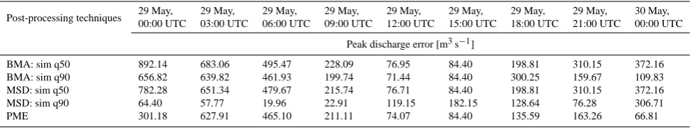
Table 3. Error in the forecast of flood discharge between observed and FEST simulated data for each time point and each post-processing tecniques in Villafranca Pellice station.

BMA: sim q50 892.14 683.06 495.47 228.09 76.95 84.40 198.81 310.15 372.16

BMA: sim q90 656.82 639.82 461.93 199.74 71.44 84.40 300.25 159.67 109.83

MSD: sim q50 782.28 651.34 479.67 215.74 76.71 84.40 198.81 310.15 372.16

MSD: sim q90 64.40 57.77 19.96 22.91 119.15 182.15 128.64 76.28 306.71

PME 301.18 627.91 465.10 211.11 74.07 84.40 135.59 163.26 66.81

In Fig. 6 MSD succeeds to correct the precipitation forecast better than BMA, while PME (Fig. 7) provides for the second peak a quite constant value in each simulation at the same level of the first.

In Figs. 8–10 flood wave estimation at Dora Riparia Susa section is shown. Simulation done using BMA precipita-tion forecast (Fig. 8) identifies the 22:00 UTC peak of 29 May and another one straight after; but forecast of this one (02:00 UTC peak of 30 May) is bigger then the real dis-charge also in short term. Disdis-charge in Fig. 9 seems to join these two peaks (10:00 p.m. of 29 May and 02:00 a.m. of 30 May). Forecast obtained by PME precipitations (Fig. 10) comes near to the rain observation one, under evaluating a lot 10:00 p.m. peak of 29 May.

Flood discharge trend in Pellice Villafranca section is showed in Figs. 11–13. Figure 11 presents the two peaks: looking at the forecast, it seems reach the highest peak at 6 am of 30 May, while the real flood wave is at 02:00 a.m. of 29 May. Discharge obtained starting from MSD rain heights reflects quite well the observed one, proving a good forecast

in the short run (3 h). Also in Fig. 13 the second peak is big-ger than the observed one, but discharge levels are lower than BMA one.

Tables 1–3 provide difference between observed and sim-ulated flood discharge for each forecast time point. Concern-ing BMA and MSD, peack discharge errors refer to 50th and 90th quantiles respectively.

6 Conclusions

On this note we intend to compare the performance of the hy-drological model when the input forecasted rain height come from three different post-processing techniques. In particular, firstly Bayesian model averaging is implemented to obtain more accurate ensemble probabilistic forecasts for rainfall fields by taking into account the particular distribution (not Gaussian) of the variables under study. Indeed, meteorologi-cal variables such as rainfall data are characterized by asym-metric distributions. Thus, full modelling is performed by

(9)

means of mixture models, where first the probability of rain is modelled and then, conditionally on the former event (it does not rain), a continuous skewed distribution is used for rainfall.

For the given test case of May 2008 flood in western Piemonte, the probabilistic discharge forecasts obtained with the Multimodel SuperEnsemble Dressing provide a good es-timation of the true observed discharges in the evolution of the event, while the results obtained with BMA and poor man ensemble are unsatisfactory.

Finally, poor man ensemble provides a mean value of de-terministic models for each time point, without taking into account observations.

The case study of May 2008 flood in western Piemonte makes a response providing an indicative information about the flood wave evolution only for short run (3 or 6 h before). Moreover, while FEST model starting from all the three post-processing techniques well estimates the first flood wave, it seems to be hard well forecast the second peak. MSD, more than BMA, seems to be able to correct its estimate making a forecast at the following time points.

Even though this work examines one singular case study with the analysis of two different and independent catch-ments, the results obtained shows the feasibility of a real time application of the hydrometeorological chain proposed and offer a starting point for further investigation addressed to a sound statistical validation of the conclusion of this memory accounting for the reanalysis of a sufficient series of different case studies.

Acknowledgements. We thank the Deutscher Wetterdienst and

MeteoSwiss for the use of their operational versions of the COSMO model in this research work. This work is partially supported by the Italian Civil Defense Department.

Edited by: L. Ferraris

Reviewed by: two anonymous referees

References

Amengual, A., Romero, R., and Alonso, S.: Hydrometeorological ensemble simulations of flood events over a small basin of Mal-lorca Island, Spain, Quart. J. Roy. Meteor. Soc., 134, 1221–1242, 2008.

Arpa Piemonte: Rapporto sull’evento alluvionale del 28–30 maggio 2008 http://www.arpa.piemonte.it/approfondimenti/ temi-ambientali/idrologia-e-neve/neve-e-valanghe/

relazioni-tecniche/analisi-eventi-meteorologici/eventi-2008/ 28 30 05Rapporto finale pt1.pdf, 2008 (in Italian).

Cane, D. and Milelli, M.: Weather forecasts with Multimodel Su-perEnsemble Technique in a complex orography region, Meteo-rol. Z., 15, 1–8, 2006.

Cane, D. and Milelli, M.: Multimodel SuperEnsemble technique for quantitative precipitation forecasts in Piemonte region, Nat. Haz-ards Earth Syst. Sci., 10, 265–273, doi:10.5194/nhess-10-265-2010, 2010a.

Cane, D. and Milelli, M.: Can a Multimodel SuperEnsemble tech-nique be used for precipitation forecasts?, Adv. Geosci., 25, 17– 22, doi:10.5194/adgeo-25-17-2010, 2010b.

Cloke, H. L. and Pappenberger, F.: Ensemble Flood Forecasting: a review, J. Hydrol., 375, 613–626, 2009.

Clyde, M.: Bayesian model averaging and model search strategies, in: Bayesian Statistics 6, edited by: Bernardo, J. M., Dawid, A. P., Berger, J. O., and Smith, A. F. M., Oxford Univ. Press, 157– 185, 1999.

Du, J., Mullen, S. L., and Sanders, F.: Short-range ensemble fore-casting of quantitative precipitation, Mon. Wea. Rev., 125, 2427– 2459, 1997.

Ebert, E. E.: Ability of a Poor Man’s Ensemble to Predict the Prob-ability and Distribution of Precipitation, Mon. Wea. Rev., 129, 2461–2480, 2001.

Hoeting, J. A., Madigan, D. M., Raftery, A. E., and Volinsky, C. T.: Bayesian model averaging: A tutorial Statistical Science Sci., 14, 382–401, 1999.

Krishnamurti, T. N., Kishtawal, C. M., Larow, T. E., Bachiochi, D. R., Zhang, Z., Williford, C. E., Gadgil, S., and Surendran, S.: Im-proved weather and seasonal climate forecasts from Multimodel Superensemble, Science, 285, 1548–1550, 1999.

Leamer, E. E.: Specification Searches: Ad Hoc Inference With Non-experimental Data, Wiley, New York, 1978.

Leith, C. E.: Theoretical skill of Monte Carlo forecasts, Mon. Wea. Rev., 102, 409–418, 1974.

Mancini, M.: La modellazione distribuita della risposta idrologica: effetti della variabilit`a spaziale e della scala di rappresentazione del fenomeno dell’assorbimento, Tesi di dottorato, Politecnico di Milano, 1990 (in Italian).

Montaldo, N., Toninelli, V., Albertson, J. D., Mancini, M., and Troch, P. A.: The effect of background hydrometeorological con-ditions on the sensitivity of evapotranspiration to model param-eters: analysis with measurements from an Italian alpine catch-ment, Hydrol. Earth Syst. Sci., 7, 848–861, doi:10.5194/hess-7-848-2003, 2003.

Montaldo, N., Ravazzani, G., and Mancini, M.: On the prediction of the Toce alpine basin floods with distributed hydrologic models, Hydrol. Process, 21, 608–621, 2007.

Priestley, C. H. B. and Taylor, R. G.: On the assessment of sur-face heat flux and evaporation using large scale parameters, Mon. Weather Rev., 100, 81–92, 1972.

Rabuffetti, D., Ravazzani, G., Corbari, C., and Mancini, M.: Ver-ification of operational Quantitative Discharge Forecast (QDF) for a regional warning system – the AMPHORE case studies in the upper Po River, Nat. Hazards Earth Syst. Sci., 8, 161–173, doi:10.5194/nhess-8-161-2008, 2008.

Raftery, A. E., Gneiting, T., Balabdaqui, F., and Polakowski, M.: Using Bayesian model averaging to calibrate forecast ensembles, Mon. Wea. Rev., 133, 1155–1173, 2005.

Ravazzani, G., Mancini, M., Giudici, I., and Amadio, P., in: Quan-tification and Reduction of Predictive Uncertainty for Sustain-able Water Resources Management, edited by: Boegh, E., Kunst-mann, H., Wagener, T., Hall, A., Bastidas, L., Franks, S., Gupta, H., Rosbjerg, D., and Schaake, J., IAHS Publ., 313, 407–416, 2007.

(10)

Sloughter, J. M., Raftery, A. E., Gneiting, T., and Fraley, C.: Prob-abilistic Quantitative Precipitation Forecasting Using Bayesian Model Averaging, Mon. Wea. Rev., 135, 3209–3220, 2007. Stefanova, L. and Krishnamurti, T. N.: Interpretation of Seasonal

Climate Forecast Using Brier Skill Score, The Florida State Uni-versity Superensemble, and the AMIP-I Dataset, J. Climate, 15, 537–544, 2002.

Stensrud, D. J., Bao, J.-W., and Warner, T. T.: Using Initial Condi-tion and Model Physics PerturbaCondi-tions in Short-Range Ensemble Simulations of Mesoscale Convective Systems, Mon. Wea. Rev., 128, 2077–2107, 2000.

Weibull, W.: A statistical distribution function of wide applicability, J. Appl. Mech.-Trans. ASME, 18, 293–297, 1951.

Zappa, M., Beven, K. J., Bruen, M, Cofiño, A. S., Kok, K., Martin, E., Nurmi, P., Orfila, B, Roulin, E., Schröter, K., Seed, A., Szturc, J., Vehviläinen, B., Germann, U., and Rossa, A.: Propagation of uncertainty from observing systems and NWP into hydrological models: COST-731 Working Group 2., Atmos. Sci. Lett., 11, 83– 91, 2010.

Ziehmann, C.: Comparison of a single-model EPS with a multi-model ensemble consisting of a few operational multi-models, Tellus, 52A, 280–299, 2000.