Applied Dynamics In School And Practice
Michael Spektor, Oregon Institute of Technology, USAWalter W. Buchanan, Texas A&M University, USA Lawrence Wolf, Oregon Institute of Technology, USA
ABSTRACT
Mechanical engineering, mechanical engineering technology, and related educational programs are not addressing in a sufficient way the principles associated with applying analytical investigations in solving actual engineering problems. Because of this, graduates do not have the adequate skills required to use the methods of applied dynamics in the process of analyzing mechanical systems. These methods allow one to obtain an understanding of the role of the parameters of a system and to carry out a purposeful control of the values of these parameters with the goal to achieve the desired performance. Engineering and engineering technology programs pay very little attention to addressing these steps. It should be stressed that these programs do not offer a universal straightforward methodology of solving linear differential equations of motion that allow revealing all important interrelationships between the aspects of the engineering problem.
It is difficult to formulate the reasons why there is such a low interest in applying the analytical approach in order to reveal the interrelationships between decisive aspects of the operational process of an engineering system in order to achieve the desired goal. Actually, there is almost a complete silence with regard to this issue. Hence, we assume that the first reason could be that there is no recognition of the existence of such a problem. In other words, there is no need to apply these analytical methods since these methods are not beneficial. We do not believe that the engineering community supports this reason. It is not a matter of demonstrating factual data that show how many times the theory was helpful. Without the support of the theory we cannot justifiably evaluate the results of our solutions. If we agree that there is problem, then why are there no publications that would stimulate discussions leading toward a solution of the problem?
Here is the second reason. Until now, engineering programs do not present the straightforward universal theoretically sound methodologies for solving the second order linear differential equations that are vital for mechanical and electrical engineering. Without any suggestions of how to solve this problem, it did not make much sense to begin a discussion. In our opinion, this is why we have silence with the regard to this problem.
However, it is well known that Laplace Transforms allow solving any linear differential equation of motion. It is justifiable to assume that the main reason why the Laplace Transform methodology is not adopted by learning environments consists in the absence of the majority of tables of Laplace Transform Pairs that are needed for solving differential equations of motion as well as differential equations describing electrical circuits. However, the situation is changed. Current publications comprise the adequate tables that are needed for solving linear differential equations of motion associated with all common mechanical engineering problems.
Practicing engineers and students need assistance in acquiring the knowledge of composing differential equations of motion. They need certain training in solving these equations using Laplace Transform methodology. Several recommendations are proposed on how to expedite the implementation in academia and in industry of the methods of applied dynamics in solving common mechanical engineering problems.
Keywords: Dynamics in Engineering; Analysis of Mechanical Systems; Control of Parameters of Engineering Systems; Differential Equation of Motion; Laplace Transforms
INTRODUCTION
sophisticated and efficient engineering solutions, avoiding unneeded intuitive testing and saving substantial amounts of time and resources. However, the acquaintance with the actual activities of practicing engineers in the areas of mechanical and electrical engineering and engineering technology indicates that analytical investigations directed to the solutions of real-life problems in dynamics have a low priority. In this time of rapidly changing and advancing technology, the analytical approach to solving real-life problems should be encouraged and considered as a necessary part of engineering activities. Revolutionary innovations, such as unmanned vehicles and drones, ect., would be impossible without intensive use of the methods of applied dynamics. Practicing engineers should have adequate skills in the implementation of these methods.
It should be clear that engineering and engineering technology graduates do not obtain adequate training in solving real-life engineering problems in dynamics. Obviously, the managerial links in industry are lacking the same training. It seems that industry does not realize that it is relevant to require academia to provide graduates with the appropriate training in the use of analytical methods. Moreover, this is probably why industry does not require inclusion of applied dynamics into the engineering and engineering technology programs. Industry and society would greatly benefit from the implementation of the analytical approach to solving real-life engineering problems. Now that the required tables of Laplace Transforms are published and the methodology of straightforward solution of the differential equation is presented in detail, there is no reason to delay the implementation of applied dynamics in academia and in industry. However, industry cannot wait until academia produces graduates having the appropriate knowledge in applied dynamics. In the best scenario, it may take a few years for academia to solve this problem. The important questions that need answers are: 1) why are students not getting adequate training in applied dynamics and 2) is it realistic to assume that engineering practitioners can become familiar with the required methods of applied dynamics in a relatively short time? This paper represents an attempt to address these questions and invites the engineering community to open a discussion regarding these issues.
APPLIED DYNAMICS IN THE WORLD OF ENGINEERING
Currently, actual engineering activities are not closely associated with the methods of applied dynamics in the processes of the development or improvement of engineering systems. However, the analytical approach represents one of the most important steps in the process of solving actual engineering problems. Ignoring this step may result in the misunderstanding of the peculiarities of working processes and accepting mistaken assumptions regarding the solutions of these problems. The wrong solution may not be just a waste of resources and time, but also may result in severe safety consequences. As an illustration to this, it is interesting to consider a real-life episode that happened in the former Soviet Union (Spektor, Wolf & Buchanan, 2016; Fall Protection in Construction, 2015). This episode presents a case of several years of work of a team of engineering practitioners led by a group of scientists developing a safety harness that was compatible with the standards of safety harnesses of all industrial countries at that time, including the USA. The results of this work were verified by applying the appropriate analysis (differential equations of motion) that lasted just several hours (not years) and performed by one person, not by a team. The verification completely discredited the outcome of the work related to this safety harness and recommended how to design the safety harness that would play its role in the required way. In fact, the safety harnesses used currently in the USA completely reflect the mentioned above recommendations.
transportation, parachuting, bungee jumping, etc.). These parameters of motion could be determined based on the analysis of a solution of a corresponding differential equation of motion.
Here is an example where applying methods of applied dynamics could be very beneficial. Many operational processes of heavy equipment such as tractors, bulldozers, excavators, tanks, etc., are associated with vibrations that are transferred to the operator’s seats. Usually these seats are supported by elastic links that are intended to decrease the influence of the vibration on the body of the operator. The corresponding analyses show that in order to minimize the vibratory action on the body of the operator the stiffness of the elastic links should be adjusted to the weight of the operator. This problem could be appropriately solved using the methods of applied dynamics.
Consider an example where the preliminary determining of the characteristics of the dynamic loading could save resources and time. Here is a typical situation that happens very often in engineering practice. It occurs that a certain machine component fails due to its insufficient fatigue strength. Usually in these cases the designers increase or reinforce the cross-sectional area of the component near failure. Then the modified component undergoes testing on a vibratory shaker (stand). The component is subject to cycling loading according to the capabilities of the shaker. The designers, as well as the testers, do not know the real characteristics of the loading factors that this component experiences in actual working conditions. Moreover, the shaker may not be able to provide the regime of loading that reproduces the actual loading. Nevertheless, the component will undergo testing anyway. If the laboratory testing is successful, the component will be installed into the actual machine for testing it in actual working conditions. Very, often, the component fails again, and the improvement cycle repeats itself. Sometimes it takes a few cycles to solve the problem. This is a very time consuming and costly procedure. Keeping in mind that the failure of the component is associated with the fatigue phenomena,it becomes clear that one cycle of testing may last at least a month. However, by using the methodologies of applied dynamics it is possible to determine the characteristics of the loading factors in a matter of days. That would allow performing the calculations of the appropriate fatigue strength resulting in a justifiable change in the design of the component. This would significantly expedite the solution of the problem and avoid essential expenses.
Here is one more example. It happened that a flexible arm bracket attached to the frame of a trailer would often fail. The attempt to increase the strength of the arm by increasing its cross-sectional area resulted in cracking of the frame near the arm. The solution of the problem was obtained by the help of methods of applied dynamics that have shown that the stiffness of the arm should be reduced in order to soften the destroying effect of the impact loading. It is possible to provide many more reasons and examples that justify the need for wider implementation of the methods of applied dynamics into the design, development, and improvement of engineering systems. In many cases the results of the analyses reveal issues that could not be predicted based on engineering experience.
TRADITIONAL EDUCATIONAL PRACTICES RELATED TO THE ANALYTICAL APPROACH
Usually the students in mechanical engineering, mechanical engineering technology and related programs are exposed to differential equations in calculus class and later in the course of dynamics. The calculus course addresses in general the structure of differential equations from the mathematical perspective and explains in a limited way some aspects of applicability of the equations to solving engineering problems. In the course of dynamics, the students acquire some knowledge about second order differential equations describing motion. At this particular time in their studies, the students do not have much understanding of engineering and technology. This is probably the main reason why it would be too early to train the students in composing differential equations of motion. This is also probably a justifiable reason why they are not getting adequate training related to the understanding the role of the parameters of an engineering system and how the interaction of these parameters could be presented by a mathematical expression.
not be solved until the famous scientist, L. Euler, based on his intuition and not on science, inserted the complex number into the solution. Therefore, it is sometimes not that simple to make a successful assumption that results in a solution of the differential equation.
COMPOSING DIFFERENTIAL EQUATIONS OF MOTION
The concept of composing differential equations of motion reflecting working processes of mechanical engineering systems and determining the loading factors applied to these systems is not presented, and probably cannot be presented in a sufficient way, in a dynamics course. This is why it is not realistic to expect that graduates would have appropriate training in applying analytical methods to solve engineering problems in dynamics upon completing this course. Composing differential equations of motion related to real-life situations is not a trivial procedure and should be taught. It should be emphasized that, in the vast majority of cases, the analysis of the solutions of differential equations of motion is based on conventional mathematical procedures and should not represent any difficulty for the graduates.
Until recently it was very difficult to find in published sources an articulated and focused description that addresses the aspects of composing differential equations of motion that reflect actual working processes of mechanical systems. This fact, by itself, represented a significant obstacle on how to introduce the methods of applied dynamics to educational programs. Recent publications (Spektor, 2014, 2015] contain adequate information regarding the appropriate steps that allow for assembling the corresponding differential equations of motion. There is no room in this article to describe the related details.
SOLVING THE DIFFERENTIAL EQUATION OF MOTION
One more essential obstacle in implementing analytical methods in educational programs is associated, in our opinion, with the absence in mechanical and related engineering programs of a universal and straightforward methodology for solving linear differential equations of motion. It is well known that in the 19th century, Pierre-Simon Laplace developed a scientifically based straightforward universal methodology that allows solving any linear differential equation of motion [Grossman & Derrick, 1968; Churchill, 1958; Bracewell, 1965). The Laplace Transforms methodology is briefly discussed in many engineering programs. Obviously, there may arise a question as to why the Laplace Transform methodology is not adopted by engineering and engineering technology programs to solve differential equations. One of the reasons is probably due to the difficulty to allocate in the framework of the undergraduate programs the required time to offer a comprehensive course in Laplace Transforms. The most important reason, in our opinion, is that it is very difficult or impossible to find in the published sources the tables of Laplace Transform Pairs that are needed to solve the majority of differential equations of motion describing common engineering problems. The vast majority of existing Laplace Transform Pairs tables, mentioned above, were developed by mathematicians for mathematicians. This situation has changed since a recently published book contains all tables of Laplace Transform Pairs that are needed for solving differential equations describing all common mechanical engineering problems (Spektor, 2015).
Several examples are presented below that briefly demonstrate the use of the Laplace Transform methodology. These examples illustrate the analysis of the solutions of certain differential equations of motion and demonstrate how to determine the characteristics of the loading factors in particular cases.
EXAMPLES OF USING THE LAPLACE TRANSFORM METHODOLOGY
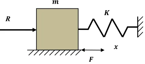
It should be emphasized that suggesting consideration of a common problem in mechanical engineering or mechanical engineering technology related to applied dynamics inevitably leads to the fact that this problem is already addressed and solved (Spektor, 2015). In the first example the requirement is to develop a system comprising a spring-loaded sliding component that is activated by a solenoid. The component is moving on a horizontal frictional surface. During the forward stroke the component is pushed or pulled by the spring-loaded solenoid. By the end of the forward stroke the component stops. The backward stroke of the component occurs due to the action of the compressed spring. The mass of the component and the length of the stroke are known. It is necessary to determine the analytical expressions that allow one to evaluate the mutual influence of the parameters of the system on each other and to calculate the values of these parameters. In analyzing this verbal formulation of the problem, it becomes clear that the motion of the component occurs due to a constant force developed by the solenoid. The forces that oppose the motion are the stiffness force exerted by the spring, the friction force between the component and the surface, and the force of inertia of the component. The air resistance in this case is negligible. Figure 1 shows the model of a system subjected to the action of a constant active force 𝑅 the stiffness force represented by a spring having the stiffness coefficient 𝐾, and a friction force 𝐹. Since the inertia force is present in all differential equations of motion there is no need to show it in the model.
Figure 1. Model of a system subjected to an active constant force, a stiffness force, and a friction force.
In this figure, 𝑚 is the mass of the component and 𝑥 is the coordinate of the component displacement. Based on the considerations presented above and accounting for the model in Figure 1, we compose the following differential equation of motion:
𝑚''*()(+ 𝐾𝑥 + 𝐹 = 𝑅 (1)
The initial conditions of motion for this case are:
for 𝑡 = 0 𝑥 = 0; ')'*= 0 (2)
where 𝑡 is the running time.
Dividing equation (1) by 𝑚 we obtain:
'()
'*(+ 𝜔2𝑥 + 𝑓 = 𝑟 (3)
𝑭
𝑲
𝒙
R
where 𝜔 is the natural frequency of the system and:
𝜔2=9
: (4)
𝑓 =:; (5)
𝑟 =:< (6)
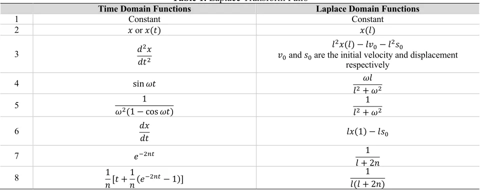
In order to use the Laplace Transform methodology, we need the table of Laplace Transform Pairs. The table below contains the pairs that are needed for solving this example. In this table 𝑙 is the complex argument in the Laplace domain.
Table 1. Laplace Transform Pairs
Time Domain Functions Laplace Domain Functions
1 Constant Constant
2 𝑥 or 𝑥(𝑡) 𝑥(𝑙)
3 𝑑2𝑥
𝑑𝑡2
𝑙2𝑥(𝑙) − 𝑙𝑣 C− 𝑙2𝑠C
𝑣C and 𝑠Care the initial velocity and displacement
respectively
4 sin 𝜔𝑡 𝜔𝑙
𝑙2+ 𝜔2
5 1
𝜔2(1 − cos 𝜔𝑡)
1 𝑙2+ 𝜔2
6 𝑑𝑥
𝑑𝑡 𝑙𝑥(1) − 𝑙𝑠C
7 𝑒L2M* 1
𝑙 + 2𝑛
8 1
𝑛[𝑡 + 1
𝑛(𝑒L2M*− 1)]
1 𝑙(𝑙 + 2𝑛)
Using the pairs 1, 2, and 3, we convert the differential equation of motion (3) with its initial conditions of motion (2) into the algebraic equation in the Laplace domain:
𝑙2𝑥(𝑙) + 𝜔2𝑥(𝑙) + 𝑓 = 𝑟 (7)
Solving equation (7) for the displacement 𝑥(𝑙) in the Laplace domain, we have:
𝑥(𝑙) =T(RLSUV( (8)
Using the pairs 1 and 5, we invert the equation (8) from the Laplace domain into the time domain and obtain the solution of the differential equation of motion (3) with its initial conditions of motion (2):
𝑥 =RLSV( (1 − cos 𝜔𝑡) (9)
In order to analyze the solution, we take the first and second derivatives from equation (9) that represents the velocity and the acceleration respectively:
') '*=
RLS
'()
'*(= (𝑟 − 𝑓) cos 𝜔𝑡 (11)
At the end of the forward stroke that lasts time T, the component stops. Equating the velocity to zero according to equation (10), we write:
0 =RLSV sin 𝜔𝑇 (12)
Since 𝑟 − 𝑓 > 0 (otherwise the solenoid would not be able to move the component), we have:
sin 𝜔𝑇 = 0 (13)
and, consequently:
𝜔𝑇 = 𝜋 (14)
Therefore:
T =VZ (15)
Combining equations (4) and (15), we obtain:
T= 𝜋[:9 (16)
Based on appropriate considerations, we accept a certain value of the time, T, which the forward stroke lasts. Thus, based on equation (16) we determine the stiffness coefficient of the spring:
𝐾 =Z\((: (17)
According to equation (14), we determine:
cos 𝜔𝑇 = −1 (18)
Combining equations (9) and (18) and accounting that at the end of the stroke the displacement of the component equals s, and also recalling the notations (4), (5), and (6), we may write:
𝑠 =2(<L;)9 (19)
Assuming that the value of the friction coefficient between the component and the surface is found in published sources, we can calculate the friction force F, and therefore, based on equation (19), we can write one more expression for the stiffness coefficient of the spring:
K = 2(<L;)] (20) Equating the right-hand sides of the equations (17) and (20), we determine the value of the constant force R, which the solenoid should apply to the component:
𝑅 =2\(;UZ2\((:] (21)
𝑅:^M= −𝑅 + 𝐹 (22)
For the stress analysis of the spring it would be reasonable to accept that the spring is subjected to a completely reversed loading cycle having the maximum force according to the following expression:
𝑅:_)= 𝑅 − 𝐹
and the minimum force according to the expression (22).
Analyzing equation (11) we determine that the maximum value of acceleration 𝑎:_) equals:
𝑎:_)= |𝑟 − 𝑓|
This concludes the analysis of the problem.
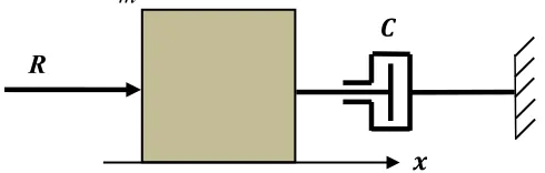
The second example is associated with calculating the maximum velocity of a submarine.
It is required to calculate the maximum velocity of a submarine in the horizontal direction that could be developed by the thrust force produced by the available source of energy. The active force applied to the submarine represents a constant force, while the resistance force is the viscous friction force of the water. The above considerations are reflected in the model presented in Figure 2, which shows a system subjected to the action of a constant active force R and a resisting viscous friction force caused by damper C.
Figure 2. Model of a system subjected to an active constant force and a viscous friction force.
Accounting the model shown in Figure 2, we compose the following differential equation of motion of the submarine:
𝑚''*()(+ 𝐶')'* = 𝑅 (23)
where 𝐶 is the damping coefficient and is the active constant force. Dividing equation (23) by 𝑚, we write:
'() '*(+ 2𝑛
')
'* = 𝑟 (24)
where 𝑛 is the damping factor, while:
2𝑛 =:c (25)
R
𝑪
𝒙
R
and
(26)
The initial conditions of motion in this case are:
For (27)
Applying the pairs 1, 2, 3, and 6, we convert the differential equation of motion (24) with its initial conditions of motion (27) into the algebraic equation in the Laplace domain:
𝑙2𝑥(𝑙) + 2𝑛𝑙𝑥(𝑙) − 𝑟 (28)
The Laplace domain solution of equation (28) reads:
𝑥(𝑙) =T(TU2M)R (29)
Based on the pair (8), we invert equation (29) into the time domain and obtain the solution of differential equation (23) with the initial conditions of motion (27):
𝑥 =2MR [𝑡 +2Me (𝑒L2M*− 1 (30)
Taking the first derivative from equation (30), we calculate the velocity of the submarine:
') '*=
R 2M1 − 𝑒
L2M* (31)
The acceleration of the submarine is determined from the first derivative of equation (31):
'()
'* = 𝑟𝑒
L2M* (32)
In this case, the velocity tends to its maximum value when the acceleration tends to zero that, according to equation (31), occurs at the following condition:
𝑒L2M*à0 (33)
Combining expressions (31) and (33) and recalling notations (25) and (26), we obtain that the maximum velocity
𝑉:_) of the submarine is determined from the following expression:
𝑉:_)→<c (34)
This concludes the solution of the example. R
r m
=
0
t= x 0; dx 0
dt
CONCLUSION
The process of solving mechanical engineering problems associated with applied dynamics comprises several steps. The following two of these steps represent certain difficulties for students and practicing engineers: 1) composing the differential equation of motion, and 2) obtaining the solution of this equation. Practicing engineers and, more so, senior and graduate students, need certain assistance in learning the principles of composing differential equations of motion for real-life mechanical engineering systems. However, the engineers and students have the adequate background in math to use the Laplace methodology in solving these differential equations. Certain assistance in this matter would be helpful. Therefore, in order to implement the methods of applied dynamics in solving actual mechanical engineering problems, it may be recommended:
1) create an appropriate course in applied dynamics for senior and graduate students and select a corresponding textbook;
2) provide short seminars for engineers and students emphasizing the aspects of composing differential equation of motion and solving them using the Laplace Transform methodology;
3) publish a compact guide for composing and solving the differential equations of motion using the Laplace Transform Pairs where a full table of the Pairs is attached to the guide;
4) place this guide on the Internet;
5) inform the engineering community in our country and in the world that all common one-degree-of-freedom mechanical engineering problems associated with linear differential equations of motion are solved and presented in the book (again, name the book, rather than just using a footnote) (Spektor, 2015), which has a guiding table for determining the needed sector in less than a minute.
AUTHOR BIOGRAPHIES
Michael Spektor graduated from Kiev Polytechnic University with a degree in Mechanical Engineering and holds a Ph.D. degree in Mechanical Engineering from Kiev Construction Engineering University in Kiev, Ukraine. He earned his professional experience in the former Soviet Union, Israel, and in the United States. He served as a Professor and Department Chair at Oregon Institute of Technology and as Program Director of Bachelor Degree Completion Degree and Master’s Degree at Boing in Seattle. He published numerous scientific papers in peer review magazines and delivered many scientific articles on national and international professional conferences. During the last five years, he published by Industrial Press the following three books: Solving Engineering Problems in Dynamics, Applied Dynamics in Engineering, and Machine Design Elements and Assemblies.
Walter Buchanan is a Past Thompson Endowed Chair Professor at Texas A&M. He has served in professorial and administrative positions at Northeastern University, Oregon Institute of Technology, Middle Tennessee State University, University of Central Florida, and Indiana University-Purdue University Indianapolis, was an electronics engineer for Naval Avionics, a Navy engineering officer, an aerospace engineer for the Boeing and Martin Companies, as well as an attorney for the Veteran’s Administration. He is a Life Fellow and served on the Board of Directors of both ASEE and NSPE, is a Fellow of ABET and IEEE, and is a Senior Member SME, and is a Past President of the Massachusetts Society of Professional Engineers. Buchanan is a member of the Board of Delegates of ABET, is on the editorial board of the Journal of Engineering Technology, has authored or co-authored over 250 publications, and has been a principal investigator for NSF grants. He is Past President of ASEE. He holds a B.S.E and M.S.E. from Purdue University, and a B.A., J.D., and Ph.D. from Indiana University. He is a registered P.E. in six states and a retired member of the Indiana State Bar.
active PE registrations in Missouri and Oregon. His international activities have included Saudi Arabia, Iran, Norway, Nigeria, Singapore and Japan.
REFERENCES
Spektor, M., Wolf, L. & Buchanan, W. (June, 2016) Implementing Applied Dynamics. In Proceedings of the2016 ASEE Annual Conference, New Orleans, Louisiana.
Fall Protection in Construction. (2015). OSHA, 3146-05R.
Spektor, M. (2014). Solving Engineering Problems in Dynamics. Connecticut:Industrial Press. Spektor, M. (2015). Applied Dynamics in Engineering. Connecticut: Industrial Press.
Grossman, S. & Derrick, W. (1968). Advanced Engineering Mathematics. New York:Harper and Row. Churchill, R. (1958). Operational Mathematics. New York: McGraw-Hill.