Geometric Modelling Of Complex Objects Using
Iterated Function System
Ankit Garg, Ashish Negi, Akshat Agrawal, Bhupendra Latwal
Abstract: In the field of computer graphics construction of complex objects is difficult process. Objects in nature are complex such as tree, plants, mountains and clouds. Traditional geometry is not adequate to describe these objects. Researchers are investigating different techniques to model such types of complex objects. Algorithms presented in this paper are deterministic algorithm and random iteration algorithm which comes under iterated function system. The fundamental property of any IFS is that image generated by it is also a fractal which is called attractor. Any set of affine transformation and associated set of probabilities determines an Iterated function system (IFS). This paper presents the role of iterated function system in geometric modeling of 2D and 3D fractal objects.
Key words: CMT, IFS
————————————————————
1
I
NTRODUCTION
Binoit Mandelbrot invented the word fractal. Latin adjective - fractus verb – frangere means ‗to break‗to create irregular fragments [12]. Fractals generated by dynamical systems are called Algebraic fractals, Ex: Mandelbrot & Julia set. In the field of computer graphics researchers are always try to find out new ways to construct geometric model of objects. Computer graphics provides various ways to construct man-made objects e.g. building, plants etc. Well developed mathematical polynomials are available to model such type of objects. These well defined mathematical polynomials can generate smooth geometry. As fractals are non smooth and highly irregular traditional polynomial methods requires more specification information. The concept of fractal was described by IBM mathematician Benoit Mandelbrot. He found that traditional geometry was inadequate to describe the structure of natural objects which are complex such as mountain, cloud, coastlines and tree. The non-Euclidean geometry or fractal geometry deals with irregular and fragmented patterns. Fractals are complex objects which has property of self similarity- A small section of fractal object is similar to whole object, hence fractal are the repetition of the same structural form. There are two main groups of fractals: linear and nonlinear [2]. The latter are typified by the popular Mandelbrot set and Julia sets, which are fractals of the complex plane [2]. Fractal may have condensation sets. Fractal with condensation set are not quite self similar. In general to create any fractal three things are required: a set of transformations (IFS), a base from which iteration starts, and a condensation set (possibly the empty set). IFS provide a very compact representation, efficient computation, and a very small amount of user specifications [1]. An IFS is a set of contraction mappings acting on a space X. The set of contraction mapping has a set of probabilities.
Construction of fractal image with IFS starts with original image and some successive transformation are applied over the image. The result of IFS is called attractor which is a fix point. This fix point after contraction mapping is nothing but an image. An IFS maps the corresponding fractal onto itself as a collection of smaller self similar copies. Seemingly a photocopy machine has been designed by mean of which coefficients of map are computed [3]. The concept of photo copy machine has also been extended to the case of gray scale images [3]. IFS can be used in fractal image compression. Barsnley has derived a special form of the Contractive Mapping Transform (CMT) applied to IFS‘s called the College Theorem. College theorem suggests that the hausdorff distance between two images should be as minimum as possible, means the attractor of IFS should be close approximation of original image. The distance between original image and attractor is known as college error and it should be as small as possible. Due to self similar property of fractal IFS is applied on whole image in fractal image compression to find out the redundancy in image. There may be some images in which only part of image is similar to the other part of image, not whole image. In this case instead of applying affine transformation on whole image, contractive affine transformations are applied on parts of image, and the union of affine transformation is the final image. This can be achieved by applying PIFS over image. Some object or classical geometry can be generated as attractor of IFS. Objects of classical geometry generated through IFS are somewhat unsatisfactory only close approximation is possible.
2
M
ATHEMATICALF
OUNDATION OFIFS
DefinitionA (hyperbolic) iterated function system consists of a complete space (X, d) together with a finite set of contraction mappings wn : X X, with respective contractivity factors sn, for n = 1, 2, ..., N. The notation for this IFS is {X ; wn, n = 1, 2, , N} and its contractivity factor is s = max{sn : n = 1, 2, , N}.
Definition
An iterated function system with probabilities [8] consists of IFS
{X; w1, w2, , wN} _________________________
Ankit Garg, pursuing PHD from Uttarakhand Technical University, Dehradun. He is working as assistant professor in Amity University, Haryana.
Ashish Negi is Associate professor in GBP Engineering College, Pauri Garhwal.
Akshat Agrawal, Pursuing PHD from Amity University, Haryana. He is working as assistant professor in Amity University, Haryana.)
2
together with an ordered set of numbers {p1, p2, , pN}, such that
p1 + p2 + p3 + + pN = 1 and pi 0 for i = 1, 2, , N.
The probability pi is associated with the transformation wi. The nomenclature IFS with probabilities may be used as an abbreviation. The full notation for such an IFS is [2].
{X; w1, w2, , wN ; p1, p2, , pN}.
The probabilities are related to the measure theory of IFS attractors, and play a role in the computation of images of the attractor of an IFS attractor using the random iteration algorithm, and also using the multiple reduction photocopy machine algorithm, as applied to grayscale images [2]. They are not used with the multiple reduction photocopy machine algorithm when it is applied to binary images [2].
Definition
The fixed point A H(X) described in the IFS Theorem is called the attractor of the IFS.
Definition
Let (X, d) be a metric space and let C H(X). Define a transformation w0: H(X) H(X) by w0 (B) = C for all BH(X). Then w0 is called a condensation transformation and C is called the associated condensation set.
Definition
Let {X; w1, w2,, wN} be a hyperbolic IFS with contractivity factor 0 s 1. Let w0: H(X) H(X) is a condensation transformation. Then {X; w0, w1,, wN} is called a (hyperbolic) IFS with condensation.
3
S
TEPS FOR CREATING FRACTAL USING IFSFor generating a fractal using iterated function system steps given below should be considered.
1. Establishing a set of transformations. 2. Draw any initial pattern on the plan.
3. Applying transformations on the initial patterns which are defined in the first step.
4. Again apply transformation on the new image which is the combination of initial pattern and pattern after applying transformations.
5. Repeat step 4 again and again, this step 4 can be repeated infinite number of times.
4
IFS
I
MPLEMENTATION4.1 The Deterministic Algorithm
This method starts with an image and apply some affine transformation on each subset of this image and try to find out next image which should be complete subset of R2 space where image lie. After applying affine transformation again and again a sequence of image will be generated which should be converging at some point which will be the limit point? This limit point is nothing but an image. This apply some mapping to get an image from other image, this mapping should be contractive. This approach to generate fractal requires heavy amount of memory, because in each iteration generate some
image and to store image generated by affine transformation requires large amount of memory.
Let {X; w1, w2,, wN} be a hyperbolic IFS. Choose a compact set A0 R2. Then compute successively An = W ° n (A) according to
An+1 = nNwj (An) for n = 1, 2, .
Thus construct a sequence {An: n = 0, 1, 2, 3,} H(X). Then by the IFS Theorem the sequence {An} converges to the attractor of the IFS in the Hausdorff metric.
4.2 The Random Iteration Algorithm
The random approach is different from the deterministic approach in that the initial set is a singleton point and at each level of iteration, just one of the defining affine transformations is used to calculate the next level. Which will also be a singleton point? At each level, the affine transformation is randomly selected and applied. Points are plotted, except for the early ones, and are discarded after being used to calculate the next value. The random algorithm avoids the need of a large computer memory, it is best suited for the small computers on which one point at a time can be calculated and display on a screen. On the other hand it takes thousand of dots to produce an image in this way that does not appear too skimpy.
Let {X; w1, w2,, wN ; p1, p2, , pN} be an IFS with probabilities. Choose x0 X and then choose recursively, independently [2], xn {w1(xn-1), w2(xn-1), , wN(xn-1)}for n = 1, 2, 3, ,where the probability of the event xn = wi(xn-1) is pi. Thus, construct a sequence {xn: n = 0, 1, 2, 3,} X.
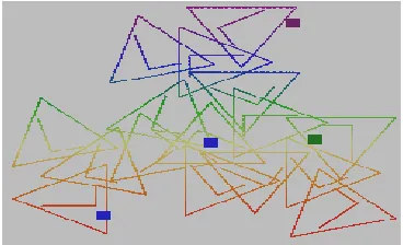
Fig 1: Design of IFS under deterministic fractal generation algorithm
Fig 3: Fractal generated after 5 iteration with four fix points
Complexity of fractal image is depending upon number of iterations.
Fig 4: Attractor of IFS after applying 18 iterations
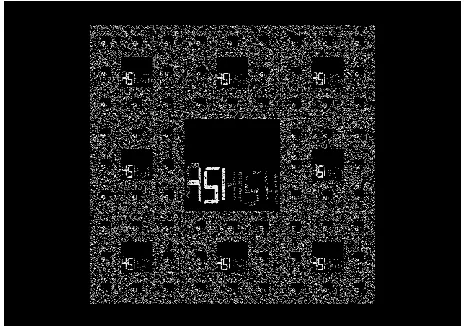
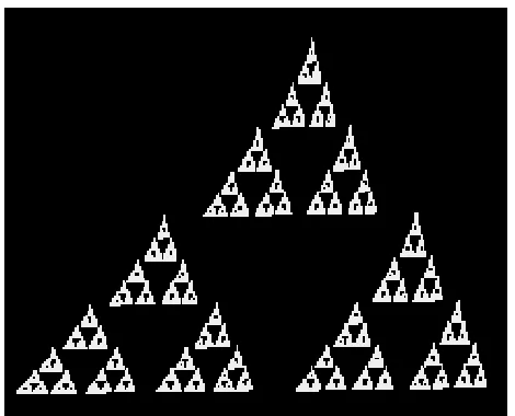
Fig 5: Fractal image after applying random fractal generation algorithm with 20 iterations
Fig 6: Fractal image after applying random fractal generation algorithm with 50 iterations
Fig 7: Attractor of IFS after applying random iteration algorithm.
5
T
HEC
OLLEGET
HEOREMTo find an IFS which results close approximation to original and attractor is called ―inverse problem". Genetic algorithm has been proposed for the inverse problem. College theorem does not solve the inverse problem but it provides some better way of approaching it. The Collage Theorem gives the idea is to find IFS whose attractor is very close approximation to the original image. The approximation or closeness of original image and attractor can be measured by using the Hausdorff metric. This result is the key to finding IFS that can be used to compress an image.
Definition
Let (X, d) be a complete metric space. Let L ∈ H (X) be given, and let �≥0 be given. Choose an IFS (or IFS with condensations){X;(W1),W2,W3,…Wn} with contractivity factor
0≤ s <1, so that ≤ ε, where h (d ) is the
4
attractor of the IFS. Equivalently
(1) For all L ∈ H(X). The collage theorem says that if D(C (T), T) <D then d(T,A) < d/(1-S), where C is an IFS with contractivity S and attractor A and T is any image. D(C (T), T) <D says that the distance between to point should be small because all the IFS should be contractive and the d(T,A) < d/(1-S) says the distance between original and attractor should be as minimum as possible or the hausdorff distance between original image and attractor should ne as minimum as possible. If the value of S close to 1, nothing ensures that this method provides a good approximation. Yet this was the original idea of Barnsley and most of the fractal based algorithm relies on the same approach. Quality of compression is depending upon how well the transformation manages to map the sections of the image in the range block to each domain block. Continuity Condition in collage theorem state that Small changes in the parameters of IFS will lead to small changes in the attractor. In other words, as the coefficients of IFS are altered, the attractor changes smoothly and without any sudden jumps [2]. In simpler terms, the Collage Theorem is stating that there are arbitrarily many IFS for the approximation of an image I, such that.
(2)
Where W (I) is called the ―Collage‖ of I. If we have a small ϵ, then we have a good approximation of I by W∞, and a large number of functions fn are necessary. On the contrary if we
have a large ε, then we have a bad approximation, where a small number of fn are sufficient. Small changes in the
parameters will lead to small changes in the attractor [9]. Rapid and even convergence to A∞, if fm (A) ⋂fn (A) is small for
m≠n, will create a good collage. Slow and uneven convergence A∞, if fm (A) ⋂fn (A) is large for, will create a bad
collage.
Fig 8: Generating Collage for fractal represented in fig 9
Fig 9: Image of attractor after applying IFS on collage
6
Q
UANTITATIVEI
NFORMATIONA
BOUTFRACTAL
I
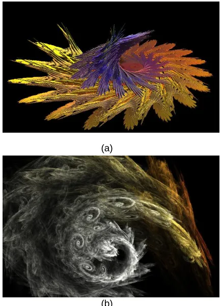
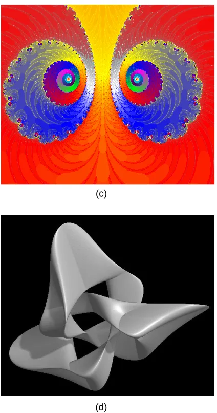
MAGESAll the pictures shown in figure 1 are generated by applying random iteration algorithm. Time taken and number of iteration to generate each picture is different from each other. The scale factor of each image tells the amount of contraction or expansion of original image. The scaling is applied after we have multiplied the points x ∈ X by the affine transformation Wi. Deterministic algorithm takes less iteration but more time
to generate picture on the other hand random iteration algorithm needs lots of iteration to generate same picture.
(a)
(b)
(c)
(d)
Fig 10: Images of fractal after applying some number of iteration (a) IFSX fractal (b) Devoured fractal (c) Face 2 Face
fractal (d) Triangular Terifoil fractal
Table 1
Quantitative information about different types of fractals images shown in section 6.
Fractal Number of
Iterations Resolution Time taken to generate the picture in Sec IFSX 200 640x480 24.742 DEVOURED 150 640X480 37.581 FACE2FACE 582 640x480 .812 TRIANGULAR
TERIFOIL 50 640x480 11.934
7
FRACTALTHEORY
AND
APPLICATIONS
Fractal geometry offers very important tools for describing and analyzing irregularity which can be classified as new regularity, seemingly random but with precise internal organization [6]. In
repeating process using a sequence of scale. Objects at each scale are indistinguishable. This feature of fractals is called self similarity. For example sierpinski triangle is obtained by successively removing triangle from initial triangle of unit side length. One of the advantages of using an iterated function system (IFS) is that the dimension of the attractor is often relatively easy to calculate in terms of the defining contractions.
8
AFFINE
TRANSFORMATION
The simplest example of iterated function system is a set of 2 dimensional affine map. 2D affine mapping has a single point. This single point is called fixed point. Fix point after applying IFS may be either stable (attractor) or unstable (repelling). System becomes unbounded with the unstable fix point because unstable fix point grows larger and larger if successive IFS apply on this point. Affine transformations are linear transformations. Affine transformation is composition of rotation, translations, dilations and shears. An affine transformation does not preserve angles or length. Two or more successive transformations can be applied on the image with the use of affine transformation.
A transformation: R2 R2 of the form
(3)
where a, b, c, d, e, and f are real numbers, is called a (two-dimensional) affine transformation. Using equivalent notations:
(4)
If IFS consists of affine contractions {S1, S2, S3 … Sn,} on ℝn
, the attractor F is called a self-affine set. Transformation in fractal geometry is contractive when it moves pair of two points closer together. Formally, a transform W is said to be contractive if for any two points P1 and P2, the distance
(5)
Where s ∈ (0, 1), and is called the contractive factor. Contractive affine transforms have the property that when they are repeatedly applied, they converge to a point which remains fixed upon further iterations.
6
9
APPLYING
DETERMINISTIC
ALGORITHM
TO
GENERATE
FRACTAL
After successively applying IFS over the initial image, final output will be an attractor which is a fractal image. The image after applying IFS in fig 5 is called self similar set because it is a union of a number of smaller self similar copies of itself.
(6)
(7)
(8)
Fig 6: Collage for constructing triangle
Fig 7: Image of fractal after applying successive IFS
10
IFS
IN
CHAOS
GAME
ALGORITHM
Suppose IFS contain M affine transformation A1, A2, A3….AM. Each affine transformation in IFS has some associated probability p1, p2, ….. pN, respectively. Affine transformation with probability is applied on chaos game algorithm. In IFS select one affine transform according to its probability and
apply to initial point (x0, yo) to find out new point (x1, y1) again apply another transform with another probability a new point (x2, y2) will be generated. Repeat this process to obtain a long sequence of points:
(x0, y0) , (x1, y1) , (x2, y2) , (x3, y3) , . . .
A basic result of the IFS theory is that this sequence of points will converge, with 100% probability, to the attractor of the IFS [7].
11
CONSTRUCTION
OF
ALGEBRIC
FRACTALS
USING
IFS
Construction of Mandelbrot Set
Fractals constructed in dynamical system are of algebraic type. Popular fractals Mandelbrot set and Julia set are generated by iterated function like f (z) = zn2 +c where z and c are complex numbers [11]. The Mandelbrot set and Julia set are also called algebraic fractals
Step 1: Input xmin, xmax, ymin, ymax, Max and Radius Where Max represents maximum number of iterations Variable Radius represents radius of the circle. Choose a simple complex function Z=x+iy and C=p+iq
x ε [xminimum, xmaximum], y ε [yminimum , ymaximum] dx =( xmaximum - xminimum)/col;
dy = (ymaximum - yminimum )/row;
Where variable col represents maximum number of columns and variable row is the maximum number of rows of the display screen.
Step 2: For all points (px, py) of the screen
(px=0, 1, 2…, col-1), (py=0,1,2,…row-1)
Go through the following routine:
Step 3: Set i=0
p0 = xmin + px * dx q0= ymin + py * dy x0 =y0=0
Step 4: Calculate (xi+1, yi+1), where xi+1and yi+1 represents real part and imaginary part respectively of given complex function.
Step 5: Compute r=xi2 + yi 2
i) If r> Radius then fill black color and go to step6 ii) If i=Max then fill white color and go to step6 iii) r<=Radius and i<Max , repeat step 4
Step 6: Plot the point (px, py, color) and go to the next point (step2).
12
CONSTRUCTION
OF
3D
OBJECTS
USING
3D
IFS
• Iteration counter
It specifies the number of point that will be iterated.
• Color mode
It specifies the color to paint the calculated point using IFS.
a) Transformation: Colors each point according to the Transformation, which have lead to it.
b) Probability: Colors each point according to the Probability, i.e. according to the previous random number.
c) Measure: Colors each pixel in the window according to how often a point hits the pixel.
Following affine matrix is required for 3D fractal image [15].
0
0
0
1
a
b
c
d
e
f
g
h
i
j
k
l
2D fractal can be generated in 3D environment by simply putting j=k=l=m=c=g=0 and taking remaining values a,b,d,e,f according to the 2D affine transformation.
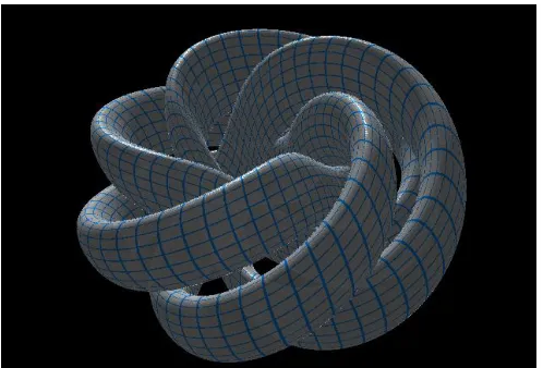
Fig 8: Construction of 3D fractal using IFS
13
DESIGN
THREE
DIMENSIONAL
COMPOUND
MODELS
In 2010, each of researcher Bulusu Rama, Jibitesh Mishra presented project on " Generation of 3D Fractal Images for Mandelbrot and Julia Sets", the 3D rendering of which gave a real-world look and felt in the world of fractal images[13]. To generate fractal shape objects a simple transformation function Z-> Z2+C will be applied to the initial set of points. This transformation function is applied on given set of points for finite number of times. The amount of detail inside fractal object is depending upon the number of iteration performed and resolution of the display system [14]. In this section design of 3D models is describe using fractal geometry and Iterated function system. The general algorithm to design 3D models is:
Step 1: select any basic model it can be sphere or cube.
Step 2: Select any shape which will be treated as additive shapes. This additive shape can be spheres or cubes or combination of both. Specify the size of additive shapes for example side length of cube and radius of sphere.
Step 3: Specify number of iterations required to design 3D compound model.
Step 4: By using Recursive function these additive shapes are drawn for a specified number of iteration in order to design 3d fractal model. To design above 3D fractal model following procedure must be follow.
1. Start with basic model i.e. sphere or it may be cube. 2. Add 3 additive shapes with the basic model. Here
additive shape is sphere. Scaling factor of each additive shape is (0.4), translation factor (ty, ty, tz) respectively is (r* 0.4, r, 0) for right sphere, (- r* 0.4, r, 0) for left sphere, (0, r, r* 0.4) for the center sphere, and rotation by X direction (angle=90). r= the radius of the sphere.
3. After some specified number of iteration, repeat step 2.
4. Result of IFS involved in generation of 3D models is an attractor which also a fractal.
Fig9: Steps of design 3D fractal model using set of spheres.
14
CONCLUSION
8
algorithm. Deterministic algorithm takes less time to generate fractal as compared to random generation algorithm. An attractor which is a fixed point after applying IFS can be stable or unstable. System becomes unbounded with the unstable fix point because unstable fix point grows larger and larger if successive IFS apply on this point. To design 3D shapes specific number of iteration, transformation (translation, rotation, reflection, scaling) of additive shapes over basic model must be defined. Complexity of 2D and 3D objects is depending upon the number of iterations.
15
ACKNOWLEDGMENTS
I thank to my guide Dr. Ashish Negi, Associate professor in Department of Computer Science and Engineering, Govind Ballabh pant Engineering College, Pauri Garhwal for providing me an opportunity and resource to carry out this work. I am also thankful to NPTEL funded by ministry of HRD government of india to carry out this work which provides E-learning through online Web and Video courses in Engineering, Science and humanities streams. I am also thankful to my wife Ayushi Garg for giving me support to carried out this work.
References
[1]. Construction of fractal objects with iterated function systems, San Francisco July 22-26.
[2]. Fractal Image Compression, Martin V Sewell, Birkbeck College, University of London, 1994.
[3]. M.F. Bernsley and L.P. Hurd. Fractal image compression. AK peters Ltd. Massachusetts, 1993.
[4]. An Introduction to Fractal Image Compression, Literature Number
[5]. BPRA065, Texas Instruments Europe October 1997
[6]. Fractal Image Compression, Martin V Sewell, Birkbeck College, University of London, 1994
[7]. Stewart. 1988. A review of: the science of fractal images, Nature 336:289.
[8]. Guojun Lu Fractal-Based Image and Video Compression The Transform and Data Compression Handbook Ed. K R. Rao et al.Boca Raton, CRC Press LLC, 2001.
[9]. Suman K. Mitra, Malay K. Kundu, C.A. Murthy, BhargabB. Bhattacharya, A New Probabilistic Approach for Fractal Based Image Compression, Fundamenta Informaticae 87 (2008) 1–17.
[10]. Julie Blue Kriska, Construction of Fractal Objects With Iterated Function Systems, MATH 547.001.
[11]. An Introduction to Fractal Image Compression, Literature Number: BPRA065, Texas Instruments Europe October 1997.
[12]. Mandelbrot. B. B, ―The Fractal Geometry of Nature‖, W. H. Freeman and Company, 1982.
[13]. Falconer,Kenneth,Techniques in Fractal Geomenty,John Willey and sons, 1997.
[14]. Rama B., Mishra j., 2010, "Generation of 3D Fractal Images for Mandelbrot and Julia Sets", ACM New York, NY, USA, Pages 235-238.
[15]. [onlineavailable]http://dspace.thapar.edu:8080/dspace /bitstream/123456789/426/1/m91536.pdf