www.solid-earth.net/4/357/2013/ doi:10.5194/se-4-357-2013
© Author(s) 2013. CC Attribution 3.0 License.
Solid Earth
An objective rationale for the choice of regularisation parameter
with application to global multiple-frequency
S
-wave tomography
C. Zaroli1, M. Sambridge2, J.-J. Lévêque1, E. Debayle3, and G. Nolet4
1Institut de Physique du Globe de Strasbourg, UMR7516, Université de Strasbourg, EOST/CNRS, France 2Research School of Earth Sciences, Australian National University, Canberra ACT 0200, Australia 3Laboratoire de Géologie de Lyon, UMR5276, CNRS, Université Lyon 1 et ENS de Lyon, France 4Géoazur, Université de Nice Sophia-Antipolis, UMR6526, CNRS, France
Correspondence to: C. Zaroli ([email protected])
Received: 4 June 2013 – Published in Solid Earth Discuss.: 28 June 2013
Revised: 29 August 2013 – Accepted: 10 September 2013 – Published: 15 October 2013
Abstract. In a linear ill-posed inverse problem, the regular-isation parameter (damping) controls the balance between minimising both the residual data misfit and the model norm. Poor knowledge of data uncertainties often makes the selec-tion of damping rather arbitrary. To go beyond that subjec-tivity, an objective rationale for the choice of damping is presented, which is based on the coherency of delay-time estimates in different frequency bands. Our method is tai-lored to the problem of global multiple-frequency tomogra-phy (MFT), using a data set of 287 078S-wave delay times measured in five frequency bands (10, 15, 22, 34, and 51 s central periods). Whereas for each ray path the delay-time es-timates should vary coherently from one period to the other, the noise most likely is not coherent. Thus, the lack of co-herency of the information in different frequency bands is ex-ploited, using an analogy with the cross-validation method, to identify models dominated by noise. In addition, a sharp change of behaviour of the model`∞-norm, as the damping becomes lower than a threshold value, is interpreted as the signature of data noise starting to significantly pollute at least one model component. Models with damping larger than this threshold are diagnosed as being constructed with poor data exploitation. Finally, a preferred model is selected from the remaining range of permitted model solutions. This choice is quasi-objective in terms of model interpretation, as the se-lected model shows a high degree of similarity with almost all other permitted models (correlation superior to 98 % up to spherical harmonic degree 80). The obtained tomographic model is displayed in the mid lower-mantle (660–1910 km depth), and is shown to be compatible with three other recent
global shear-velocity models. A wider application of the pre-sented rationale should permit us to converge towards more objective seismic imaging of Earth’s mantle.
1 Introduction
2010). To better constrain the structure of the Earth’s inte-rior, new theoretical developments on seismic wave propa-gation have emerged in recent years, and received increas-ing attention in tomography. Dahlen et al. (2000) developed an FF approach (hereafter referred to as banana–doughnut theory, BDT) that is efficient enough to be applied to large-scale problems and a wide range of frequencies. It is based on a ray–Born approximation that is much faster than the mode summation approaches proposed earlier by Marquer-ing et al. (1998) and Zhao and Jordan (1998). We refer the reader to Sect. 1.6 of Nolet (2008) for more complete ref-erences to work preceding Dahlen et al. (2000). To go be-yond tomographic limitations from ray-based FF kernels of BDT (e.g. Nolet, 2008), alternatives are available (e.g. Zhao et al., 2000; Tromp et al., 2005; Nissen-Meyer et al., 2007; Zhao and Chevrot, 2011a, b). The most promising ones are based on numerical techniques (e.g. Komatitsch et al., 2002) and the adjoint method (e.g. Tarantola, 1987; Tromp et al., 2005). Such large scale tomographic applications are cur-rently limited to periods greater than∼50 s, where the dom-inant part of the signal corresponds to surface waves (e.g. Fichtner et al., 2009; Tape et al., 2010; Lekic and Romanow-icz, 2011). Mercerat and Nolet (2012) investigate the ac-curacy of BDT delay-time predictions and conclude that, even though errors withVSkernel predictions are larger than
those forVP, the errors remain well below typical
observa-tional uncertainty, while the kernels computed this way re-quire two to three orders of magnitude less CPU time. In the past 10 yr, various applications of BDT have shown in-teresting tomographic results (e.g. Montelli et al., 2004b, 2006; Hung et al., 2004; Yang et al., 2006, 2009; Sigloch et al., 2008; Sigloch, 2011; Sigloch and Mihalynuk, 2013; Nolet, 2009; Tian et al., 2009, 2011). In parallel, several stud-ies questioned whether the benefits from using BDT, rather than simple RT, could be smaller than the uncertainty posed by the subjective regularisation of the inverse problem (e.g. Sieminski et al., 2004; Trampert and Spetzler, 2006; Van der Hilst and de Hoop, 2005; Boschi et al., 2006). It seems per-tinent that tomographers ask what are the consequences on seismic models of the subjectivity inherent to the choice of regularisation parameter. Linear tomographic inverse prob-lems, d=Gm, are usually ill-posed and require a subjec-tive degree of regularisation to deal with data errors and sta-bilise the solution. One usually uses Tikhonov regularisation (Tikhonov, 1963), which consists in solving the minimisa-tion problemmλ=arg min(||d−Gm||2
2+λ 2||m||2
2), where λis a real regularisation parameter (damping) to be chosen with care. A convenient and widely used graphical tool (e.g. Aster et al., 2012) for setting the dampingλis to analyse the trade-off curve (L curve) between the model norm (||m||2
2, squared Euclidean norm) and the data misfit (χred2 , reduced chi-square). In a tomographic experiment, data errors are a mix of observational and modelling errors. Ideally, if the statistics of data errors would perfectly be known, the
op-timal solution would be reached forχred2 '1 near the bend of theLcurve. In practice this is never met, as data errors are usually just best guesses, and one faces the dilemma to choose a solution around theLcurve’s corner as a best com-promise between minimising both the residual data misfit and the model norm. Therefore, the selection of an optimally regularised solution is to a large extent arbitrary – more akin to an art form – which can lead to different model interpreta-tions. To converge towards more reliable tomographic mod-els, one would prefer to lessen the inherent subjectivity of the damping choice. The goal of this study is to present a new approach aimed at objectifying the choice of regularisation parameter in the case of global multiple-frequency tomogra-phy (MFT, equivalent to BDT applied in multiple-frequency bands, as named by Sigloch et al., 2008). We will illustrate our approach using a global data set of 287 078 shear-wave delay times measured at 10, 15, 22, 34 and 51 s central pe-riods (Zaroli et al., 2010). To summarise, our approach will consist of the following three parts: (i) identifying models with poor data exploitation (over-damped); (ii) identifying models dominated by noise (under-damped); and (iii) select-ing a preferred model among the remainselect-ing ones. We will show that this final choice is of no consequence in terms of model interpretation, and thus is quasi-objective. The pre-ferred model we obtain this way will be displayed in mid lower-mantle (660–1910 km depth), where our data coverage is at its highest. We will briefly discuss its major structural features, and show its compatibility with three other, latest generation, global shear-velocity models.
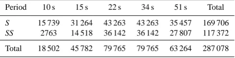
2 Global multiple-frequencyS-wave tomography 2.1 A global data set of multiple-frequencyS-wave
delay-times
We use a globally distributed data set of 287 078 S and
SS delay-times measured at 10, 15, 22, 34 and 51 s periods
Table 1. Global data set of multiple-frequency shear-wave delay-times.
Period 10 s 15 s 22 s 34 s 51 s Total
S 15 739 31 264 43 263 43 263 35 457 169 706 SS 2763 14 518 36 142 36 142 27 807 117 372 Total 18 502 45 782 79 765 79 765 63 264 287 078
ω−α, with anαvalue of 0.2 for S and 0.1 for SS .” Thus, S and
SS delays are corrected for physical dispersion by injecting
thoseαvalues in Eq. (16) of Zaroli et al. (2010). After correc-tion for physical dispersion due to 1-D attenuacorrec-tionq(ω)and crustal reverberations, the data exhibit a residual dispersion of the order of 1–2 s in the 10–51 s period range. Zaroli et al. (2010) suggest that this residual dispersion is partly related to seismic heterogeneities in the mantle. For instance, they show that wavefront-healing phenomenon (e.g. Gudmund-son, 1997) is clearly observed for S waves having passed through negativeVSanomalies. Tian et al. (2011) show that
the inclusion of additional dispersion due to 3-D attenuation structure has little influence onS-wave models. Sigloch et al. (2008) show that one can neglect it forP-waves, and, sim-ilarly, Savage et al. (2010) observe only a small effect on seismic wave travel times. Thus, we neglect the role of 3-D variations of attenuation to explain the residual dispersion in our data. Bolton and Masters (2001) extensively discuss the assignment of quantitative errors in the case of a global S wave data set. Following their analysis, we aim at identify-ing the separate contributions to the total data varianceσT2in our data set. We have: σT2=σ32−D+σX2+σN2, where σ32−D is due to 3-D seismic heterogeneities, σX2 is due to earth-quake location errors, andσN2 is attributed to measurement errors. Bolton and Masters (2001) estimateσXfor S waves to be 1.6–2.5 s, assuming a typical depth uncertainty of about 10 km, at epicentral distances of about 70◦, and for misloca-tion vectors of length 10–20 km. In this study, we have at-tributed to each datumdia constant value for the source
un-certaintyσX=2.5 s. Earthquake mislocation and origin time effects are not simultaneously estimated for each datum dur-ing the inversion. In addition, we assume that the source un-certainty is the same for anS-wave measured at either 10, 15, 22, 34, or 51 s period, so that taking it into account would not change the main results of this study. Moreover, Masters et al. (2000) report that their tomographic results of S wave inversions vary little when source effects are included. As for the contribution of the measurement error, we have at-tributed to each datumdian individual error{σN}icomputed
with Eq. (9) of Zaroli et al. (2010). It varies between 0.1 and 3.7 s, though its average value is 0.49, 0.57, 0.67, 0.73, and 1.08 s for data subsets at 10, 15, 22, 34, and 51 s periods, re-spectively. Thus, the total data uncertaintyσi for each datum
di isσi=(σX2+ {σN}2i)
1/2.
2.2 Setting up the inverse problem
At each period a waveform is influenced by a weighted aver-age of Earth’s mantle through its corresponding 3-D sensitiv-ity kernel. In principle, measuring the delay-time of a seismic phase at several periods should increase the amount of inde-pendent information in the inverse problem, and lead to im-proved tomographic imaging. The general form of the MFT inverse problem is
δti(T )=
Z
Vi(T )
Ki(r;T )m(r)d3r, (1)
where δti(T ) is the time residual of target seismic phase
i measured in a passband with dominant wave period T. The volume Vi(T ) is limited to the region where the
am-plitude of the sensitivity (Fréchet) kernelKi(r;T )is
signif-icant. The model parameterm(r)represents a velocity per-turbation with respect to the 1-D reference velocity model IASP91 at each pointr in the medium. This linear inverse problem can be formulated asd=Gm, whered andmare vectors of data (sizeN) and model parameters (sizeM), re-spectively. The G sensitivity matrix (sizeN×M) is the pro-jection of the Fréchet kernels onto the model parameterisa-tion. In Appendices A and B, we expand on the computa-tion of (i) the data-driven model parameterisacomputa-tion, and (ii) the “analytical” ray-based FF kernels. For more details, in-cluding for the computation of G, we refer the reader to Zaroli (2010). In order to solve this linear inverse prob-lem, we assume that the prior covariance matrices of the data, Cd, and of the model parameters, Cm, follow Gaussian probability functions. Thus, we may obtain the maximum-likelihood estimate of the model solution by minimising (e.g. Tarantola and Nercessian, 1984; Tarantola, 1987):f (m)= (Gm−d)tC−d1(Gm−d)+mtC−m1m; which leads to solving a system of normal equations:
C−d1/2G C−m1/2
!
m=
C−d1/2d
0
. (2)
For each source–receiver pair, uncertainties associated with delays should partially be correlated at different periods. For instance, because of common errors on source location and origin time. So that the matrix Cd should contain off-diagonal terms. However, for simplicity, we use a off-diagonal data covariance matrix of the form: Cd=diag(σi2)1≤i≤N.
Tomographic inverse problems are usually ill-posed and re-quire a degree of regularisation to deal with data errors and stabilise the solution. The model covariance, Cm, represents our prior expectation of how model parameters are corre-lated, e.g. high correlation for nearby parameters. We use a simple model covariance of the form: Cm=σm2IM, where
integrate over a volume as wide as several Fresnel zones, a simple regularisation parameter (damping) λ=1/σm is sufficient, in our experience, to obtain smoothed solutions. Setting G0=C−d1/2G andd0=C−1/2
d d, one can write (Eq. 2) as
G0 λIM
m=
d0 0
. (3)
To solve the weighted, damped least-squares problem (Eq. 3), we use LSQR (Paige and Saunders, 1982), an iterative row action method that converges to solution
mλ= arg min(||d0−G0m||2
2+λ2||m||22). Care has been taken to ensure LSQR convergence with sufficient iterations. After a first inversion with zero damping, outliers with data mis-fit deviations larger than±3σ were rejected for subsequent inversions. Total amount of surviving data is N=287 078 (cf., Table 1). Let us defineχ2=PN
i=1({d0}i− {G0mλ}i)2=
PN
i=1({d}i− {Gmλ}i)2/σi2. It is a direct measure of the data
misfit, in which we weight the misfits inversely with their standard errors. In the perfect case that data are on aver-age satisfied with a misfit of one standard deviation, we findχ2'N, so that it is convenient to define the reduced chi square χred2 =χ2/N. As always, the crucial choice of dampingλcontrols the balance between both minimising the model norm||m||2
2and data misfitχ 2
red. In the following, we present an objective rationale for the choice ofλthat is tai-lored to the MFT problem.
3 An objective rationale for the choice of damping The MFT inverse problem (Eq. 1) is ill-posed in the sense that, in absence of regularisation, small changes in the data can lead to large changes in the computed model solution. This forces us to impose some sort of regularisation of the problem to filter out the noise effects, which leads to solv-ing (Eq. 3). The big question is how to choose the regu-larisation parameter (damping λ) that gives an appropriate balance between filtering out enough noise without losing structural information. To converge towards more reliable to-mographic images, there is a need to significantly lessen the subjectivity associated to the damping choice. Not doing so could prevent us from correctly mapping into the model the weakS-wave delay-time dispersion observed in our global data set. First, let us define some useful notations. LetdT
be the data subset with central periodT, MBλ the multi-band model from inversion ofd10,15,22,34,51 with damping λ, SBλ340 the single-band model from inversion of d34 with damping λ0, and χred2 (m,dT)the misfit ofdT with model
m. Perhaps the most convenient and widely used graphi-cal tool for setting the damping is theL curve analysis. It usually consists in analysing the curve of trade-off between the size of the model (e.g. measured by||m||2
2) and the data misfit (e.g. measured byχred2 ). One usually gets a charac-teristic L-shaped curve, with a (not often distinct) corner
separating “vertical” and “horizontal” parts of the curve. Figure 1 shows the curve of trade-off between ||MBλ||2 2 andχred2 (MBλ,d10,15,22,34,51). One sees that the model with data misfitχred2 (MBλ,d10,15,22,34,51)=1 is probably under-damped as it lies on the quasi-vertical leg of the L curve. This indicates that this model is dominated by noise, as will be confirmed in Sect. 3.2, and is a reminder of our imperfect knowledge of the statistics of data errors (σi). Our estimates
of σi appear to be slightly under-estimated, which may be
caused by non-Gaussian distributions of source and measure-ment uncertainties. It is possible to estimate observational er-rors of teleseismic waves using the concept of summary rays (e.g. Morelli and Dziewonski, 1987; Gudmundsson et al., 1990). However, the problem is larger for MFT, since very little experience so far is at hand on the observational error sources (e.g. crustal reverberations) that affect narrow-band cross-correlation estimates. Hansen and O’Leary (1993) sug-gest that the optimal damping could be the one maximising theLcurve’s curvature (maximum curvature criterion). Be-cause of some intrinsic arbitrariness in this criterion, it should be applied with caution (e.g. Boschi et al., 2006). For in-stance, theLcurve has to be a plot of un-dimensional quanti-ties, by scaling both data and model to prior uncertainty. We compute the curvature asκ(λ)=(ρ0η00−ρ00η0)/(ρ02+η02)3/2, whereη= ||MBλ||2
2, andρ=χred2 (MB
λ,d
10,15,22,34,51). We
normaliseηandρ by their extrema values. The prime and double prime mean the first and second derivative with re-spect toλ, respectively. Figure 1 shows the plot of curvature κin function of data misfit, superimposed to theLcurve plot. The multi-band model maximisingκ is shown with a black diamond marker, and is named MBκmax. In Sect. 3.2, we
will identify MBκmax as part of models dominated by noise.
Hansen and O’Leary (1993) also suggest that the maximum curvature criterion may yield an under-damped solution if theLcurve is characterised by a “smooth” corner, as it is in our case. Finally, there is a wide range of models with ac-ceptable data misfit around theLcurve bend. Picking one of them is to a large extent arbitrary. This motivates us to de-velop, for the MFT problem, a more objective approach to determine an “optimal range” of damped solutions. It will primarily consist in identifying models with “poor data ex-ploitation” or “dominated by noise”, as summarised in Fig. 1 and explained below.
3.1 Identifying multi-band models with poor data exploitation
Fig. 1. Summary of our approach for objectifying the choice of regularisation parameter (damping). We plot the curve of trade-off (Lcurve) between the model norm,||MBλ||2
2, and its residual data misfit,χred2 (MBλ,d10,15,22,34,51), as dampingλvaries. The
Lcurve is displayed with solid-line parts in blue, red and light or-ange, corresponding to different model ranges. Its curvatureκ is shown with a grey dashed line (with arbitrary amplitude scaling). The model MBκmax (black diamond) corresponds to the maximum
curvature of theLcurve. The two extreme models MBnoise and MBpoordelimit the range of models “dominated by noise” or “with poor data exploitation”, respectively. In Sect. 3.3, we show that the selection of our preferred model MBpref (black star), from the re-maining “optimal range” of permitted models, can be qualified as quasi-objective.
||mλ||2=(PM j=1|mλj|
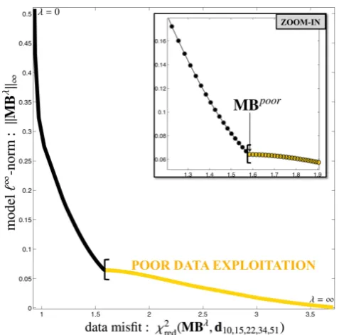
2)1/2. However, it corresponds to an L curve with a very smooth corner, as shown in Fig. 1. To render this smooth corner sharper, one may analyse a new L curve based on the model `∞-norm: ||mλ||∞= max(|{mλ}j|)1≤j≤M. We further refer to this new trade-off
curve as the L∞ curve. It simply is an alternative evalua-tion of the size of regularised models plotted in funcevalua-tion of data misfit. Figure 2 shows this curve of trade-off between ||MBλ||∞ and χred2 (MBλ,d10,15,22,34,51). As expected, the
corner of the L∞curve has been sharpened by the`∞-norm, but it is interesting to see that two regimes are now apparent on both sides of a breaking point. Letλpoorbe the damping value for which this change of regime occurs, and MBpoorbe the corresponding multi-band model. Figure 2 shows that as the dampingλdecreases down to the critical valueλpoor, the `∞-norm (i.e. the largest model component) increases very gently. One sees that as soon as the damping gets smaller than this critical value, then at least one model component starts to behave differently: its amplitude is suddenly more
Fig. 2. Plot of the curve of trade-off between the model`∞-norm,
||MBλ||∞, and its residual data misfit,χred2 (MBλ,d10,15,22,34,51). A sharp change of behaviour of the model`∞-norm occurs as the dampingλgets lower than a threshold valueλpoor, which is inter-preted as the signature of data noise starting to significantly pollute at least one model component. Models with dampingλ≥λpoorare identified as with “poor data exploitation”.
increased while the data misfit continues to decrease. Since the `∞-norm is equal to the model parameter with largest amplitude, it easily detects the presence of at least one noisy model component with unrealistic high amplitude. In con-trast, Fig. 1 shows a smooth increase of the`2-norm of mod-els slightly less damped than the critical model MBpoor. This is due to the fact that the`2-norm reflects integrated informa-tion over all model parameters, and is less sensitive to a sin-gle noisy parameter. Therefore, we interpretλpooras being the smallest damping value for which no model component is significantly contaminated by noise. The damping range corresponding to poor data exploitation is then defined by λ≥λpoor (where poor stands for “poor data exploitation”). We have visually checked that tomographic models within this range of damping do not seem to be deteriorated by noise. Finally, as one aims at exploiting the most of our data set (e.g. structural dispersion due to wavefront healing), it may be rewarding to consider models with a better fit to data than for MBpoor, which motivates us to identify models dom-inated by noise.
in different frequency bands (10, 15, 22, 34, and 51 s central periods). That is, for each ray path, the structural information should be coherent from one period to the other, but the noise information most likely not. In the following, using a form of cross-validation method, we show that the lack of coherency of the information in different frequency bands can be ex-ploited to identify models dominated by noise.
3.2.1 Identifying single-band models dominated by noise
The first step is to identify a range of single-band models, SBλ340 (inversion of 34 s data subset,d34, with dampingλ0), which are “dominated by noise”. Our approach consists in testing how well single-band models fit the 10 s data subset (d10), as damping varies. The philosophy of this approach is somewhat analogous to the cross-validation (CV) method, in that we aim at estimating the fit of a model (SBλ340) to a data set (d10) that is similar but not identical to the data (d34) that were used to derive the model. However, our data partitioning approach markedly differs from the random subdivision of data inherent in CV. Partition into frequency bands, based on similar sensitivities to mantle structure, seems to make more sense in the context of our multi-frequency data set.
Figure 3 shows the corresponding curve of trade-off be-tween the model norm, ||SBλ340||2
2, and its 10 s data misfit, χred2 (SBλ340,d10). This trade-off curve is not L shaped any-more, but is characterised by a remarkable “reversal”. Let λ0noise be the damping value corresponding to this reversal, and SBnoise34 be the associated model. One sees that the more the dampingλ0is decreased beyond the critical valueλ0noise, the more the single-band model gets complex (increase of ||SBλ340||2
2) while its 10 s data misfit gets poorer (increase ofχred2 (SBλ340,d10)). We interpret as dominated by noise the range of single-band models, SBλ340, with dampingλ0≤λ0noise (where noise stands for “dominated by noise”). Indeed, for large values of dampingλ0one expects smooth single-band models giving similar data predictions at all periods. As one decreases the dampingλ0 into the domain where we are fit-ting the noise more than the structure-imposed trend in the 34 s data, one expects that single-band models will fail to satisfy the 10 s data, because the 10 and 34 s data noise should not be coherent. Therefore, we consider SBnoise34 as the most damped single-band model among those obviously dominated by noise. As a consequence, the range of single-band models with damping “slightly larger” thanλ0noisemust somehow be significantly polluted by noise. This may in-tuitively be understood when looking at the inset in Fig. 3. The more the damping decreases towards λ0noise, the more the trade-off curve becomes vertical, i.e. decreasing the 10 s data misfit costs very much in terms of model norm increase. A priori, one ignores what is the most expensive cost that is affordable, so that one cannot objectively identify this range of models with significant noise contamination, i.e. before
Fig. 3. Illustration of the coherency analysis. It consists in testing how well single-band models, SBλ340 (inversion of 34 s data), fit the 10 s data (d10) as dampingλ0 varies. The curve of trade-off be-tween the single-band model norm,||SBλ340||2
2, and its 10 s data mis-fit,χred2 (SBλ340,d10), is characterised by a “reversal” which occurs for dampingλ0noise. Single-band models with dampingλ0≤λ0noise
are identified as “dominated by noise”.
the noise predominant regime. However, its existence will be taken into account for the choice of the preferred model (Sect. 3.3).
3.2.2 Inferring multi-band models dominated by noise from single-band models
Fig. 4. Illustration showing how to infer multi-band models domi-nated by noise from single-band models. The curve of trade-off, be-tween model norm and 34 s data misfit, is plotted for single- (SBλ340, dashed line) and multi-band (MBλ, solid line) models. An accept-able multi-band model should not give a better fit to the 34 s data (d34) than the single-band model SBnoise34 . Thus, multi-band models withχred2 (MBλ,d34)≤χred2 (MBnoise,d34)are identified as “dom-inated by noise”. The multi-band model MBnoiseis defined as hav-ing the same 34 s data misfit as SBnoise34 .
For completeness, the coherency analysis should be ap-plied to all combinations of single-band models and fit of data subsets. The relatively low number of 10, 15, and 51 s data (cf. Table 1) restricted us to analyse single-band models derived from either 22 or 34 s data. To do this, we imposed the same source–receiver geometry for multi- and single-band (22 or 34 s) models, so that differences between models cannot be due to this extraneous factor. We analysed single-band models, SBλ340 (or SBλ220), with their fit to the 10, 15, 22 (or 34), and 51 s data subsets, respectively. Corresponding Lcurve reversals were reached for different values of damp-ing,λ0, which mainly reflects, at each period, the data noise level and the sensitivity kernel. We observed that the analysis of models derived from the 34 s data, and their fit to the 10 s data subset, lead to identify the narrowest range of accept-able multi-band models. Thus, for clarity, Sect. 3.2 has been focussed on this case.
3.3 Quasi-objective choice of preferred multi-band model
We have identified an optimal range (cf. Fig. 1) of multi-band models MBλwith dampingλnoise< λ < λpoor. The next step
consists in choosing a “preferred” model MBpref among those candidates, i.e. in between the two extreme models MBnoiseand MBpooras illustrated in Fig. 5a. Picking a par-ticular solution within this range is a matter of compromise between exploiting most of the structural information (small damping) and minimising noise influence (large damping). One cannot avoid some subjectivity concerning this ultimate choice. Thus, one needs to estimate if this degree of subjec-tivity can still lead to significant model differences in terms of structural interpretation. We do this by looking at the level of correlation between the candidate solutions.
Figure 5b and d shows the correlation of models MBλ[
960,1510] from the optimal range with respect to the two extreme models MBnoise[
960,1510]and MB poor
[
960,1510], respectively, where [960,1510] means that we only consider
a vertical average of a model over depth range 960–1510 km. The correlation is displayed for spherical harmonic degrees l=1–80. The characteristic horizontal length associated with degreel=80, in this particular depth range, is about 400 km. We checked that all correlation results were simi-lar if considering any other depth range through the man-tle. From hereon, for ease of notation, we drop the|[960,1510] subscript on models. The correlation is computed as follows: letSA(l)=(Plm=−lAml A
m∗
l )1/2be the spectrum of a given
square-integrable functionAdefined on the unit sphere, with Aml the spherical harmonic coefficients at degreel and az-imuthal order m, and ∗ the complex conjugate. The cor-relation between two such functions A and B is defined as Corr(A, B;l)=Pl
m=−lAml B m∗
l /(SA(l)SB(l)). Figure 5b
and d shows that every model within the optimal range has a correlation coefficient larger than ∼91 %, up to degree l=80, with respect to the two extreme models. This indi-cates that this optimal range contains highly similar models, in terms of shear-velocity anomaly patterns. Thus, selecting any of them would lead to a similar structural interpretation. However, it seems to us wiser to choose the preferred model MBpref as better correlated to MBpoor (not significantly in-fluenced by noise) than to MBnoise(dominated by noise). To support this choice, note that models slightly more damped than MBnoise, though not quantitatively identified, are cer-tainly polluted by noise as suggested at the end of Sect. 3.2.1. Figure 5c shows that our preferred model MBprefhas a cor-relation coefficient larger than∼98 %, up to degreel=80, with respect to almost every model within the optimal range (excepted those too close from MBnoise). Obviously, such small model differences are not relevant, so that our choice of a preferred solution can be qualified as quasi-objective.
4 Looking at mid lower-mantle through multiple-frequencyS-wave delay-times
Fig. 5. Illustration showing that the selection of our preferred multi-band model MBpref(black star) is quasi-objective in terms of model in-terpretation. (a) Trade-off curve corresponding to the “optimal range” of models, after identification of those “dominated by noise” (MBnoise) or with “poor data exploitation” (MBpoor).(b–d) Plot of the correlation of three specific models (MBnoise, MBpref, MBpoor, as indicated by white arrows) with several models MBλspanning the “optimal range” of models (respectively). Correlation is shown for spherical harmonic degreesl=1–80, and is displayed using the colour scale on the right (black is 100 %, and white is 98 %). One sees that MBprefhas a corre-lation coefficient greater than 98 %, up to degreel=80, with respect to almost all models MBλwithin the optimal range. The characteristic horizontal length associated withl=80 is∼400 km. Here, the correlation is shown for models averaged over 960–1510 km depth, but we checked that it holds true at other depths.
simultaneous inversion of a global data set of 287 078 S and SS delay-times measured by cross-correlation in five fre-quency bands (10, 15, 22, 34, and 51 s central periods). Tech-nical tomographic details are given in Sect. 2 and in Appen-dices A and B. The construction of such a model was mo-tivated by the recent discovery of significant structural dis-persion in this data set, after correction for crustal and 1-D attenuation effects. Taking into account this new observ-able global tomography holds the promise to better constrain the structure of Earth’s interior. Our current data coverage is too sparse below∼2000 km depth, owing to the drastic criteria applied by Zaroli et al. (2010) for cross-correlating fully isolated S and SS waveforms only. For instance, S waves
major structural features in our model, and show its com-patibility with three other recent global shear-wave velocity models. We postpone a detailed structural interpretation of our tomographic results, which is beyond the scope of this paper.
Figure 6 displays our model MBpref between 660 and 1910 km depth. One can see long wavelength, high-velocity anomalies concentrated in the circum-Pacific and regions un-der Asia, as widely documented in the past (e.g. Li and Ro-manowicz, 1996; Masters et al., 1996; Grand et al., 1997; Van der Hilst et al., 1997; Masters et al., 2000; Ritsema and Heijst, 2000; Megnin and Romanowicz, 2000; Romanowicz, 2003; Montelli et al., 2004a, b, 2006; Houser et al., 2008; Rit-sema et al., 2011). Geodynamicists now widely agree upon a link between these broad-scale anomalies and cold down-wellings from ancient subductions driving an important part of the mantle circulation (e.g. Schuberth et al., 2009). For in-stance, one sees the seismic signature of the ancient Farallon slab beneath North America (e.g. Grand et al., 1997), and of the remnants of Tethys beneath the Mediterranean/southern Eurasia (e.g. Van der Hilst and Karason, 1999; Houser et al., 2008). They are usually associated with cold material sink-ing into the lower mantle. Concernsink-ing the Farallon slab, it is worth noting that our model features at 960–1510 km depth a detached slab beneath the western quarter of North Amer-ica (Fig. 6d), as recently discussed by Sigloch and Miha-lynuk (2013). The presence of two large low-velocity re-gions at the core–mantle boundary, beneath Africa and the Pacific, is a common feature found in previously cited whole-mantleS-wave models. These two regions are often referred to as superplumes, and could be feeding up smaller low-velocity anomalies in the mid lower-mantle (e.g. Davaille, 1999; Davaille et al., 2005; Courtillot et al., 2003; Lay, 2005; Montelli et al., 2006; Schuberth et al., 2009). Figure 6 shows that some of them are apparent in our model, most often be-neath Africa and the Pacific and generally located near to a known hotspot (Tahiti, Samoa, Horn of Africa, Afar, South Africa, etc).
Figures 6 and 7 show that long-wavelength structures, which are very similar across recent tomographic models (e.g. Romanowicz, 2003), are well retrieved in this study. More precisely, Fig. 7 shows for visual comparison our model MBpref with three other, latest generation, global shear-velocity models: S40RTS (Ritsema et al., 2011), PRI-S05 (Montelli et al., 2006), and TX2007 (Simmons et al., 2007). S40RTS results from Rayleigh wave phase velocity, teleseismic shear-wave travel time and normal mode split-ting function measurements, and is parameterised by spher-ical harmonics up to degree 40 and by 21 vertspher-ical spline functions. PRI-S05 and MBprefresult from cross-correlation shear-wave delay times measured in one or several frequency band(s), respectively. They are irregularly parameterised ac-cording to data coverage. TX2007 results from a joint in-version of seismic data (teleseismic shear-wave travel times) and geodynamic constraints (global free-air gravity, tectonic
Fig. 6. Tomographic maps of shear-velocity anomalies of our model MBpref at selected depths in mid lower-mantle: 660– 960, 960–1510, and 1510–1910 km depth. Black lines: continents; green lines: tectonic plates; green circles: hotspots (Anderson and Schramm, 2005).
Fig. 7. Visual comparison of our model (MBpref, left column) with three other global shear-velocity anomaly tomographic models (S40RTS, PRI-S05, TX2007), displayed in mid lower-mantle with respect to IASP91 and after projection onto our model parameterisation.
Fig. 8. (a–c) Spectral amplitude as a function of spherical harmonic degreel=1–50 for four tomographic models in mid lower-mantle: our model MBpref (black), S40RTS (blue, plotted up tol=40), PRI-S05 (red), and TX2007 (green). (d–f) Correlation as a function of degreelbetween our model MBprefand the three other models: S40RTS (blue), PRI-S05 (red), and TX2007 (green). The black dashed- and solid-lines indicate the 95 and 66 % significance levels, respectively.
subjective amount of regularisation used in the inversion. In the case of global MFT, we have shown how to strongly lessen this subjectivity, and hence counteract our poor knowl-edge of data uncertainties. A broader use of this philosophy could help to converge towards more objective seismic imag-ing of the mantle, which could strengthen the comparison of different tomographic models.
5 Conclusions
regularisation parameter (damping). Poor knowledge of data uncertainties often makes the selection of damping rather ar-bitrary, which leaves the choice of optimum model to the in-vestigator. This issue is even more important for MFT, since to date there exists little understanding of the observational error sources that affect narrow-band cross-correlation esti-mates. To go beyond that subjectivity, an objective rationale for the choice of damping in the case of MFT has been pre-sented and validated using a large data set of 287 078S-wave delay-times measured in five frequency bands (10, 15, 22, 34, and 51 s central periods). First, we have shown how to take advantage of the expected coherency of delay-time estimates in different frequency bands. That is, whereas for each ray path the delay-time estimates should vary coherently from one period to the other, the noise most likely is not coherent. Thus, we have shown that the lack of coherency of the infor-mation in different frequency bands could be exploited, us-ing an analogy with the cross-validation method, to identify models dominated by noise (under-damped). In addition, we have shown that analysing the behaviour of the model`∞ -norm, as damping varies, could give us access to the signa-ture of data noise starting to significantly pollute at least one model component, and thus could help us to identify models constructed with poor data exploitation (over-damped). We have shown that the selection of a preferred model from the remaining range of permitted solutions, i.e. models neither dominated by noise nor with poor data exploitation, could be qualified as quasi-objective. Indeed, the selected model shows a high degree of similarity with almost all other per-mitted models (correlation superior to 98 % up to spherical harmonic degree 80). For completeness, the resulting tomo-graphic model has been presented at selected depths in mid lower-mantle (660–1910 km depth), and shown to be com-patible with three other recent global shear-velocity models. In conclusion, we believe that the presented rationale, for ob-jectifying the choice of damping, could benefit various styles of the inverse problem. For instance, the coherency analysis could easily be applied to other data types, provided that data could be subdivided into subsets with similar sensitivity to model parameters – as we did when subdividing our multi-band data set into single-multi-band subsets. A wider application of this rationale should help to converge towards more ob-jective seismic imaging of Earth’s mantle, and thus to better understand its dynamics.
Appendix A
Multi-resolution model parameterisation based on spherical triangular prisms
We assume that the whole-mantle shear-wave model is de-scribed by a finite number of parameters(mj)1≤j≤M. Thus,
the continuous model is given by m(r)=PM
j=1mjbj(r),
where the basis functions, bj, represent the model
Fig. A1. Illustration of the model parameterisation. (a) 18 constant-depth spherical layers used for radially parameterising the mantle. (b) Optimised node distribution (black triangles mesh) obtained in one layer (530–660 km depth). The nodes agency attempts to fit a “resolution length” function, ranging in this case from 210 (magenta) to 850 km (cyan), that is driven by data coverage. (c) Representation of a spherical triangular prism, where the red dots represent three nodes of the model grid.
Appendix B
Analytical expressions for finite-frequency ray-based sensitivity kernels
We aim at deriving analytical expressions for single-phase (KS, KSS) and two-phase interference (KS+sS, KSS+sSS)
kernels, in order to decrease the computational cost of banana-doughnut kernels (Dahlen et al., 2000). This is valu-able as we aim at computing hundreds of thousands of ker-nels on a very fine grid (regular cells with edges of 20 km); and it may be useful for double-checking the validity of nu-merical calculations. Examples of such analytical kernels are displayed in Fig. B1. The finite-frequency delay-time sensi-tivity kernel of a single-phase, with respect to velocity per-turbation (δc/c), is (Dahlen et al., 2000)
K(rx)= − 1 2π c(rx)
Rrs
crRxrRxs
N (18) D
N (18)= ∞
R
0
ω3| ˙m(ω)|2sin[ω1T −18]dω
D= ∞
R
0
ω2| ˙m(ω)|2dω,
(B1)
whererx is the spatial position of scatterer x, 18 is the
phase shift due to passage through caustics or super critical reflection,Rrs,Rxr,Rxs are the geometrical spreading
fac-tors,| ˙m(ω)|2is the source power spectrum,1T is the detour time of the scattered wave,cr and c(rx)are the velocities
at receiver and scatterer position, respectively. Earthquake catalogues contain a large majority of shallow earthquakes, which implies to take into account the interference of a
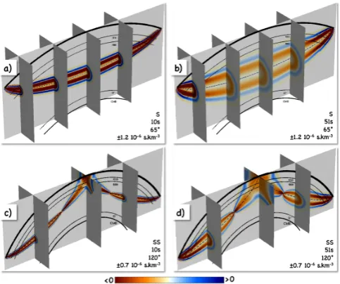
di-Fig. B1. Three-dimensional view of “analytical” ray-based finite-frequency delay-time sensitivity kernels. Each subfigure provides the phase name (S or SS), the dominant wave period (10 or 51 s), the epicentral distance (65◦for S, 120◦for SS), and the colour scale bounds (s km−3). The source is at the surface, and the black dashed line represents the geometrical ray path.
rect phase (e.g. S, SS) with its associated depth phase (e.g. sS,
sSS) within the cross-correlation time window. The kernel
K1+2(rx)= −2π c(1rx)N1+D21(18)+2
N1+2(18)= ∞
R
0
ω3| ˙m(ω)|2[· · · ]1+2dω [. . .]1+2= [. . .]11+ [. . .]12+ [. . .]21+ [. . .]22 [. . .]11=
√
|det(H1)|sin(ω1T1−18)
[. . .]12=√|det(H1)|sin(ω(1T1+t1−t2)−18) [. . .]21=√|det(H2)|sin(ω(1T2+t2−t1)−18) [. . .]22=√|det(H2)|sin(ω1T2−18)
D1+2= ∞
R
0
2(1+cos(ω(t1−t2)))ω2| ˙m(ω)|2dω,
(B2)
where “1” and “2” stand for the direct and depth phases, and whereti,1Ti, and Hi are the predicted arrival times, detour
times, and Hessian matrices of the direct (i=1) and depth (i=2) phases, respectively. Provided the filtered source time functionm(t ) has a known analytical expression, one sees that it is possible to calculate analytical expressions for both single- and two-phase interference kernels. We only need to calculate the ratios of integrals overωin Eqs. (B1) and (B2); the remaining terms can easily be computed using the soft-ware by Tian et al. (2007), available at: https://www.geoazur. net/GLOBALSEIS/Soft.html. Thus, following Hung et al. (2001), we assume a Gaussian filtered source time function whose spectrum is given by | ˙m(ω)|2=ω2T2
2π e
−ωT
2π
2
, with T the dominant wave period. This assumption is appropri-ate forS-waves within the 10–51 s period range. Unless the wave is super-critically reflected, with an angle-dependent phase shift,18takes three possible values: 0,−π/2, and −π. For S waves, 18 is always equal to 0, while for SS waves18= −π/2 in between the two caustics and18=0 elsewhere. Equations (B1) and (B2) neglect the effects of transmission coefficients as well as directional effects in the scattering, which are small as long as the sensitivity kernel is narrow. Thus, the maximum detour time1T to which we compute the kernel is equal toT (wave dominant period), which neglects third and higher order Fresnel zones. The re-sulting analytical expressions we obtain for single-phase ker-nels (KS,KSS) are
N (18=0)=16π10√π1T
T9e
− 1T π T 2
1T4−5 T 1Tπ 2
+15 4
T π
4
N 18=−π 2
=T2
2π
25 π T
10
1T4−9 2
T 1T π
2
+2 Tπ4
−25√π π T
11
1T e−
π 1T
T 2
1T4−5 T 1T π 2 +15 4 T π 4
erfi π 1TT
D=6π32 π
T
3
.
(B3)
For two-phase interference kernels (KS+sS, KSS+sSS), we
find
N1+2(18=0)=
√
|det(H1)|(I (1T1)+I (1T1+t1−t2)) +√|det(H2)|(I (1T2)+I (1T2+t2−t1))
I:x→e−(xπT)
2
H5 xπT √π πT6
H5:x→32x5−160x3+120x (Hermite polynomial of order 5) N1+2 18=−π2
=√|det(H1)|(J (1T1)+J (1T1+t1−t2)) +√|det(H2)|(J (1T2)+J (1T2+t2−t1))
J:x→25 πT10 x4−9
2 xT
π 2
+2 Tπ4
−25√π πT11xe−(xπT)
2
x4−5 xTπ2+15 4
T π
4 erfi xπT
D1+2=12π 3 2 π
T 3
+2γ (t1−t2)
γ:x→8π32 π T
7 e−(xπT)
2
x4−12 xT2π2
+12 2πT4 .
(B4)
We use the derived Maclaurin series expansion for the evalu-ation of the imaginary error function, which is
erfi(z)=√2 π
z
Z
0
e+t2dt=√2 π
∞
X
n=1
z2n−1
(2n−1)((n−1)!). (B5) The numerical approach of Simpson et al. (2003) is used to estimate the numbernof terms needed for the series to con-verge. We find that n=10 is appropriate in our case. For completeness, note that for compound rays (sS, SS, sSS), one scatterer can, sometimes, be associated to more than one per-pendicular projection point on the geometrical ray path (e.g. Hung et al., 2000; Tian et al., 2007; Nolet, 2008). Thus, for scatterers near a discontinuous interface, such as the surface, we made sure to take into account incoming rays that hit the scatterer directly as well as those that first visit a boundary.
Acknowledgements. The authors thank the Iris and Geoscope data
centres for providing seismological data, the young researcher ANR TOMOGLOB no. ANR-06-JCJC-0060 and the SEISGLOB ANR 2011 Blanc SIMI 5-6-016-01, the ERC (Advanced grant 226837) and a Marie Curie Re-integration grant (project 223799). Discussions with A. Maggi and B. S. A. Schuberth have been stimulating at various stages of this research. The authors thank M. Obayashi and K. Yoshizawa for helpful reviews that improved the original paper.
Edited by: K. Liu
References
Anderson, D. L. and Schramm, K. A.: Global hotspot maps, in: Plates, Plumes and Paradigm, edited by: Presnall, D. and An-derson, D., G. S. of America, 2005.
Aster, R. C., Borchers, B., and Thurber, C.: Parameter Estimation and Inverse Problems, Elsevier, 2012.
Bassin, C., Laske, G., and Masters, G., The Current Limits of Res-olution for Surface Wave Tomography in North America, EOS Trans AGU, 81, F897, 2000.
Boschi, L., Becker, T. W., Soldati, G., and Dziewonski, A. M.: On the relevance of Born theory in global seismic tomography, Geo-phys. Res. Lett., 33, L06302, doi:10.1029/2005GL025063, 2006. Chapman, C.: A new method for computing synthetic seismograms,
Geophys. J. Roy. Astr. Soc., 54, 481–518, 1978.
Courtillot, V., Davaille, A., Besse, J., and Stock, J.: Three distinct types of hotspots in the Earth’s mantle, Earth Planet. Sc. Lett., 205, 295–308, 2003.
Dahlen, F. A., Hung, S.-H., and Nolet, G.: Fréchet kernels for finite-frequency traveltimes – 1. Theory, Geophys. J. Int., 141, 157– 174, 2000.
Davaille, A.: Simultaneous generation of hotspots and superswells by convection in a heterogenous planetary mantle, Nature, 402, 756–760, 1999.
Davaille, A., Stutzmann, E., Silveira, G., Besse, J., and Cour-tillot, V.: Convective patterns under the Indo-Atlantic box, Earth Planet. Sc. Lett., 239, 233–252, 2005.
Debayle, E., Kennett, B. L. N., and Priestley, K.: Global azimuthal seismic anisotropy and the unique plate-motion deformation of Australia, Nature, 433, 509–512, 2005.
Dziewonski, A. M. and Anderson, D.: Preliminary reference Earth model, Phys. Earth Planet. Inter., 25, 297–356, 1981.
Fichtner, A., Kennett, B. L. N., and Igel, H.: Full waveform tomog-raphy for upper-mantle structure in the Australasian region using adjoint methods, Geophys. J. Int., 179, 1703–1725, 2009. Fukao, Y., Widiyantoro, S., and Obayashi, M.: Stagnant slabs in
the upper and lower mantle transition region, Rev. Geophys., 39, 291–323, 2001.
Grand, S. P., Van der Hilst, R. D., and Widiyantoro, S.: Global seis-mic tomography: a snapshot of convection in the Earth, GSA To-day, 7, 1–7, 1997.
Gudmundson, O.: On the effect of diffraction on traveltime mea-surement, Geophys. J. Int., 124, 304–314, 1997.
Gudmundsson, O., Davies, J. H., and Clayton, R. W.: Stochastic analysis of global travel time data: mantle heterogeneity and ran-dom errors in the ISC data, Geophys. J. Int., 102, 25–44, 1990. Hansen, C. and O’Leary, D.: The use of the L-curve in the
regular-ization of discrete ill-posed problems, SIAM J. Sci. Comput., 14, 1487–1503, 1993.
Houser, C., Masters, G., Shearer, P. M., and Laske, G.: Shear and compressional velocity models of the mantle from cluster anal-ysis of long-period waveforms, Geophys. J. Int., 174, 195–212, 2008.
Hung, S.-H., Dahlen, A., F., and Nolet, G.: Fréchet kernels for finite-frequency traveltimes – 2. Examples, Geophys. J. Int., 141, 175– 203, 2000.
Hung, S.-H., Dahlen, F. A., and Nolet, G.: Wavefront-healing: a banana-doughnut perspective, Geophys. J. Int., 146, 289–312, 2001.
Hung, S.-H., Shen, Y., and Chiao, L.-Y.: Imaging seismic velocity structure beneath the Iceland hotspot: a finite-frequency approach, J. Geophys. Res., 109, B08305, doi:10.1029/2003JB002889, 2004.
Kennett, B. and Engdahl, E.: Traveltimes for global earthquake lo-cation and phase identifilo-cation, Geophys. J. Int., 105, 429–465, 1991.
Komatitsch, D., Ritsema, J., and Tromp, J.: The spectral-element method, Beowulf computing and global seismology, Science, 298, 1737–1742, 2002.
Lay, T.: The deep mantle thermo-chemical boundary layer: the pu-tative mantle plume source, Geological Society of America, Spe-cial Paper 388, 2005.
Lekic, V. and Romanowicz, B.: Inferring upper-mantle structure by full waveform tomography with the spectral element method, Geophys. J. Int., 185, 799–831, 2011.
Li, X. D. and Romanowicz, B.: Global mantle shear velocity model developed using nonlinear asymptotic coupling theory, J. Geo-phys. Res., 101, 22245–22272, 1996.
Marquering, H., Nolet, G., and Dahlen, F. A.: Three-dimensional waveform sensitivity kernels, Geophys. J. Int., 132, 521–534, 1998.
Masters, G., Johnson, S., Laske, G., Bolton, H., and Davies, J. H.: A shear-velocity model of the mantle, Philos. T. Roy. Soc. A, 354, 1385–1411, 1996.
Masters, G., Laske, G., Bolton, H., and Dziewonski, A. M.: The relative behaviour of shear velocity, bulk sound speed and com-pressional velocity in the mantle: implications for chemical and thermal structure, in: Earth’s Deep Interior, edited by: Karato, S., Forte, A., Liebermann, R. C., Masters, G., and Stixrude, L., AGU, 63–88, 2000.
Megnin, C. and Romanowicz, B.: The 3-D velocity structure of the mantle from the inversion of body, surface, and higher mode waveforms, Geophys. J. Int., 143, 709–728, 2000.
Mercerat, E. D. and Nolet, G.: Comparison of ray- and adjoint-based sensitivity kernels for body-wave seismic tomography, Geophys. Res. Lett., 39, doi:10.1029/2012GL052002, 2012. Michelini, A.: An adaptive-grid formalism for traveltime
tomogra-phy, Geophys. J. Int., 121, 489–510, 1995.
Montelli, R., Nolet, G., Dahlen, F. A., Masters, G., Engdahl, E. R., and Hung, S.-H.: Finite-frequency tomography reveals a variety of plumes in the mantle, Science, 303, 338–343, 2004a. Montelli, R., Nolet, G., Masters, G., Dahlen, F. A., and Hung,
S.-H.: Global P and PP traveltime tomography: rays versus waves, Geophys. J. Int., 158, 636–654, 2004b.
Montelli, R., Nolet, G., A., Dahlen, F. A., and Masters, G.: A catalogue of deep mantle plumes, new results from finite-frequency tomography, Geochem. Geophy. Geosy., 7, Q11007, doi:10.1029/2006GC001248, 2006.
Morelli, A. and Dziewonski, A. M.: Topography of the core-mantle boundary and lateral homogeneity of the liquid core, Nature, 325, 678–683, 1987.
Nissen-Meyer, T., Dahlen, F., and Fournier, A.: Spherical-earth Fréchet sensitivity kernels, Geophys. J. Int., 168, 1051–1066, 2007.
Nolet, G.: A Breviary of Seismic Tomography, Cambridge Univer-sity Press, Cambridge, UK, 2008.
Nolet, G.: Slabs do not go gently, Science, 324, 1152–1153, 2009. Nolet, G. and Montelli, R.: Optimum parameterization of
tomo-graphic models, Geophys. J. Int., 161, 365–372, 2005.
Paige, C. C. and Saunders, M.: LSQR: An algorithm for sparse, linear equations and sparse least squares, ACM T. Math. Softw., 8, 43–71, 1982.
Rawlinson, N., Pozgay, S., and Fishwick, S.: Seismic tomography: a window into deep Earth, Phys. Earth Planet. Inter., 178, 101– 135, 2010.
Ritsema, J., van Heijst, H.-J., and Woodhouse, J. H.: Complex shear wave velocity structure imaged beneath Africa and Iceland, Sci-ence, 286, 1925–1928, 1999.
Ritsema, J., Deuss, A., van Heijst, H.-J., and Woodhouse, J. H.: S40RTS: a degree-40 shear-velocity model for the mantle from new Rayleigh wave dispersion, teleseismic traveltime and normal-mode splitting function measurements, Geophys. J. Int., 184, 1223–1236, 2011.
Romanowicz, B.: Global mantle tomography: progress status in the past 10 years, Annu. Rev. Earth Planet Sci., 31, 303–328, 2003. Sambridge, M. and Rawlinson, N.: Seismic tomography with
ir-regular meshes, in: Seismic Earth: Array Analysis of Broadband Seismograms, edited by: Levander, A. and Nolet, G., AGU, 157, 49–65, 2005.
Savage, B., Komatitsch, D., and Tromp, J.: Effects of 3-D attenua-tion on seismic wave amplitude and phase measurements, Bull. Seism. Soc. Am., 100, 1241–1251, 2010.
Schuberth, B. S. A., Bunge, H.-P., and Ritsema, J.: Tomographic fil-tering of high-resolution mantle circulation models: can seismic heterogeneity be explained by temperature alone?, Geochem. Geophy. Geosy., 10, Q05W03, doi:10.1029/2009GC002401, 2009.
Sieminski, A., Lévêque, J.-J., and Debayle, E.: Can finite-frequency effects be accounted for in ray theory surface wave tomography?, Geophys. Res. Lett., 31, L24614, doi:10.1029/2004GL021402, 2004.
Sigloch, K.: Mantle provinces under North America from multi-frequency P wave tomography, Geochem. Geophy. Geosy., 12, Q02W08, doi:10.1029/2010GC003421, 2011.
Sigloch, K. and Mihalynuk, M.: Intra-oceanic subduction shaped the assembly of Cordilleran North America, Nature, 496, 50–56, doi:10.1038/nature12019, 2013.
Sigloch, K. and Nolet, G.: Measuring finite-frequency body-wave amplitudes and traveltimes, Geophys. J. Int., 167, 271–287, 2006.
Sigloch, K., McQuarrie, M., and Nolet, G.: Two-stage subduction history under North America inferred from multiple-frequency tomography, Nat. Geosci., 1, 458–462, 2008.
Simmons, N. A., Forte, A. M., and Grand, S. P.: Thermochemical structure and dynamics of the African superplume, Geochem. Geophy. Geosy., 12, L02301, doi:10.1029/2006GL028009, 2007.
Simmons, N. A., Myers, S. C., and Ramirez, A.: Multi-resolution seismic tomography based on recursive tessellation hierarchy, in: Proceedings of the 2009 Monitoring Research Review: Ground-Based Nuclear Explosion Monitoring Technologies, 1, 211–220, 2009.
Simpson, M. J., Clement, T. P., and Yeomans, F. E.: Analyti-cal model for computing residence times near a pumping well, Ground Water, 41, 351–354, 2003.
Spakman, W. and Bijwaard, H.: Optimization of cell parameteri-zations for tomographic inverse problems, Pure Appl. Geophys., 158, 1401–1423, 2001.
Tape, C., Liu, Q., Maggi, A., and Tromp, J.: Seismic tomography of the Southern California crust based upon spectral-element and adjoint methods, Geophys. J. Int., 180, 433–462, 2010.
Tarantola, A.: Inversion of traveltimes and seismic waveforms, in: Seismic Tomography, edited by: Nolet G., Reidel, Dordrecht, 135–157, 1987.
Tarantola, A. and Nercessian, A.: Three-dimensional inversion without blocks, Geophys. J. Roy. Astr. Soc., 76, 299–306, 1984. Tian, Y., Montelli, R., Nolet, G., and Dahlen, F. A.: Computing traveltime and amplitude sensitivity kernels in finite-frequency tomography, J. Comp. Phys., 226, 2271–2288, 2007.
Tian, Y., Sigloch, K., and Nolet, G.: Multiple-frequency SH-tomography of the western US upper mantle, Geophys. J. Int., 178, 1384–1402, 2009.
Tian, Y., Zhou, Y., Sigloch, K., Nolet, G., and Laske, G.: Structure of North American mantle constrained by simultaneous inversion of multiple-frequency SH, SS, and Love waves, J. Geophys. Res, 116, B02307, doi:10.1029/2010JB007704, 2011.
Tikhonov, A.: Solution of incorrectly formulated problems and the regularization method, Dokl. Akad. Nauk. SSSR, 151, 501–504, 1963.
Trampert, J. and Spetzler, J.: Surface wave tomography: finite fre-quency effects lost in the null space, Geophys. J. Int., 164, 394– 400, 2006.
Tromp, J., Tape, C., and Liu, Q.: Seismic tomography, adjoint meth-ods, time reversal and banana-doughnut kernels, Geophys. J. Int., 160, 195–216, 2005.
Van der Hilst, R. D. and de Hoop, M. V.: Banana-doughnut kernels and mantle tomography, Geophys. J. Int., 163, 956–961, 2005. Van der Hilst, R. D. and Karason, H.: Compositional heterogeneity
in the bottom 1000 km of Earth’s mantle: toward a hybrid con-vection model, Science, 283, 1885–1888, 1999.
Van der Hilst, R. D., Widiyantoro, S., and Engdahl, E. R.: Evidence for deep mantle circulation from global tomography, Nature, 386, 578–584, 1997.
Yang, T., Shen, Y., van der Lee, S., Solomon, S., and Hung, S.-H.: Upper mantle beneath the Azores hotspot from finite-frequency seismic tomography, Earth Planet. Sci. Lett., 250, 11–26, 2006. Yang, T., Grand, S., Wilson, D., Guzman-Speziale, M.,
Gomez-Gonzalez, J., Dominguez-Reyes, T., and Ni, J.: Seismic structure beneath the Rivera subduction zone from finite-frequency seismic tomography, J. Geophys. Res., 114, B01302, doi:10.1029/2008JB005830, 2009.
Zaroli, C.: Global multiple-frequency S-wave tomography of the Earth’s mantle, Ph.D. thesis, Strasbourg University, 2010. Zaroli, C., Debayle, E., and Sambridge, M.: Frequency-dependent
effects on global S-wave traveltimes: wavefront-healing, scatter-ing and attenuation, Geophys. J. Int., 182, 1025–1042, 2010. Zhao, L. and Chevrot, S.: An efficient and flexible approach to the
calculation of three-dimensional full-wave Fréchet kernels for seismic tomography – 1: Theory, Geophys. J. Int., 185, 922–938, 2011a.
Zhao, L. and Chevrot, S.: An efficient and flexible approach to the calculation of three-dimensional full-wave Fréchet kernels for seismic tomography – 2: Numerical results, Geophys. J. Int., 185, 939–954, 2011b.
Zhao, L. and Jordan, T.: Sensitivity of frequency dependent trav-eltimes to laterally heterogeneous, anisotropic structure, Geo-phys. J. Int., 133, 683–704, 1998.

![Figure 5b and d shows the correlation of models960����two extreme models��[,1510] from the optimal range with respect to the MBnoise9601510 and MBpoor9601510,](https://thumb-us.123doks.com/thumbv2/123dok_us/110699.1511351/7.595.51.288.62.295/figure-correlation-models-extreme-optimal-respect-mbnoise-mbpoor.webp)