Nonparametric Confidence Interval for Quantiles

(1)

Mohammad Bolbolian Ghalibaf

Department of Statistics, Faculty of Mathematics and Computer Sciences Hakim Sabzevari University, Sabzevar, Iran

Abstract

Quantiles, which are also known as values-at-risk in finance, frequently arise in practice as measures of risk. Confidence intervals for quantiles are typically constructed via large sample theory or the sectioning.

One of the ways for achieving the confidence interval for quantiles is direct use of a central limit theorem. In this approach, we require a good estimator of the quantile density function. In this paper, we consider the nonparametric estimator of the quantile density function from Soni et al. (2012) and we obtain confidence interval for quantiles. In the following, by using simulation, the coverage probability and mean square error of this confidence interval is calculated. Also, we compare our proposed approach with alternative approaches such as sectioning and jackknife.

Keywords: Bandwidth, Jackknife Estimator, Kernel Function, Nonparametric Confidence Interval, Quantile Density Function, Quantile Function, Sectioning.

1. Introduction

The quantile function _Q _F1_{associated with a distribution function}

F defined as

1

( ) ( ) inf{ ; ( ) }, for 0 1, Q u F u  x F x u  u

is sometimes the object of more direct interest than the F itself. The use of quantiles spans a wide range of fields, especially in finance, which are known as values-at-risk, nuclear engineering and project planning (Nakayama, 2012).

Assuming F has a positive derivative F x( )f x( ) on its domain, define 1

( ) ( ) ,

( ( )) q u Q u

f Q u 

 

to be the quantile density function by Parzen (1979), and earlier dubbed the sparsity index

by Tukey (1965). The quantile density function is of much practical relevance mainly because it appears as part of the asymptotic variance of empirical quantiles.

The basic concept for deriving the confidence Interval (CI) for quantiles is well known. The first time Woodruff (1952) presented a method for estimating a CI for quantiles. The approach consists of three steps: a point estimate of the cumulative distribution function, a CI for the point estimate, and converting it into CI for the quantile.

(2)

estimate of the variance of the point estimate. The last attempt is to apply a jackknife approach to reducing the bias of previously method (based on sectioning).

In this paper, we consider the first approach and by using nonparametric estimator of the quantile density function introduced by Soni et al. (2012) construct a CI for quantile. Then we compare results of three methods numerically.

The layout of the paper is as follows: In Section 2, we express three methods to achieve CI for quantile. In Section 3, we represent smooth estimator of the quantile density function from Soni et al. (2012) and using it construct a CI for quantile. Section 4 contains the results of the simulation. In this section, we compare coverage probability (CP), mean square error (MSE) and the expected length of CI in our introduced approach with those in two other approaches. The conclusion is given in Section 5 and all tables appear in the appendix.

2. Confidence Interval Attempts

In the following we will review three attempts to achieve CI for quantiles.

2.1. Direct use of a CLT

A common approach to developing a CI is to first show that the quantile estimator satisfies a CLT, and then replace the variance constant in the CLT with a consistent estimator of it to construct a CI. We will use this approach to introduce nonparametric CI for quantile. For this purpose, we use the CLT for quantile estimator from Serfling (1980).

Suppose X₁,,Xn be

n

identically independent distribution (i.i.d.) random variables

from a distribution F and X(1)X( )n be the order statistics corresponding to 1, , n

X  X . Let F xn( ) be the usual empirical distribution function, i.e.,

1

( ) ( ),

n

n i

i

F x I X x

n 







the sample estimator corresponding to Q u( ) is defined by

1

( ) ₍ 1_{, ]} 1

ˆ ( ) ( ) ( ), for 0 1.

n

n n i i i

i n n

Q u F u X I  u u



 



 

Serfling (1980) shows that Q uˆ ( )n is asymptotically normal with mean Q u( ) and variance 2

n 

, where

(1 )

(1 ) ( ). ( ( ))

u u

u u q u f Q u

    

This leads to a large sample 100(1)% CI for quantile Q u( ) of the form

1 2

ˆ ( )n

Q u z n

 





(3)

Unfortunately, this CI is not implementable in practice since q u( ) is typically unknown, and then so is . If we have a consistent estimator for q u( )(i.e., q u_n( )q u( ) as n ), then we can replace  in Equation (1) by Sn  u(1u q u) n( ) to obtain

1 2

ˆ ( ) n ,

n

S Q u z

n

 



as another approximate 100(1)% CI for quantile Q u( ).

Generality, in this method there are two sources of error to build the CI for Q u( ). The first source, estimator of the quantile function and another source, estimator of the quantile density function. To view the various estimators for the u-th quantile refer to Steitnberg (1983). The estimation of the quantile density function for the first time have been suggested by Siddiqui (1960) and studied by Bloch and Gastwirth (1968), Bofinger (1975), Reiss (1978), Sheather and Maritz (1983), Babu (1986), Falk (1986), Welsh (1988), Jones (1992), Soni et al. (2012) and Chesneau et al. (2016).

2.2. Sectioning

Sectioning or batching is a very general methodology for constructing CI for a performance measure . All the performance measures considered thus far in the course can be handled via the use of sectioning (for a detailed discussion of sectioning see Lewis and Orav, 1988). To illustrate the idea, suppose that we wish to construct a CI for quantile Q u( ). We suppose that the total number of independent replications n of our simulation experiment takes the form nmk , where mcorresponds to the number of sections. Think of m as being relatively small (say 10 to 20), with the number of observations k per section being very large.

Let Q_{n i}_{( )}( )u be the estimator for quantile Q u( ) based on all the observations



X _j : (i1)k  1 j ik



associated with the i-th section. Observe that the estimators

(1)( ), , ( )( )

n n m

Q u Q u are i.i.d. (since each estimator is based on a statistically identical, independent section of observations). By the previous CLT,

2

( )( ) ~ ( ), 1 ,

D

n i i

Q u N Q u for i m

k 

 

 

   

where the normal random variables N1.,Nm are independent. In other words, the

section estimators Qn(1)( ),u ,Qn m( )( )u behave, for large n (or equivalently, large k ),

like i.i.d. normal random variables with mean Q u( ) (the quantity we wish to estimate) and unknown variance

2

k 

. Therefore if n is large (so that the CLTs are good

approximations), it follows that an approximate 100(1)% CI for quantile Q u( ) is

1,1 2

,

n

n _m

V Q t

m

  



(4)

( ) 1 2 ( ) 1 1 . 1 ( ) . 1 m

n n i

i m

n n i n

i

Q Q

m

V Q Q

m      



and 1,1 2 m t _

  is percentile (1 ₂)



 from Student-t distribution with m1 degrees of freedom.

Remark 1. It is important, in using the above Student-t CI, to use the divisor m1

(rather than m) in computing Vn, because the number of sections m will typically be relatively small.

2.3. The Jackknife Estimator and Sectioning

ˆ

n

Q and Qn in CLT and sectioning methods are two estimators of quantile Q u( )

respectively, but Qn has a bias that is roughly $m$ times as large as that of Qˆn. The large

bias of Qn makes it an undesirable estimator for quantile Q u( ) and renders this approach

to constructing CI for quantile Q u( ) unsuitable without some further modification. We can apply a jackknife approach to reducing the bias of previously described CI methodology based on sectioning (for more details see Lewis and Orav (1988) and Nelson (1990)).

Suppose that Q_n be the sample estimator for Q u( ) based on all n observations and ( )

n

Q i% be the sample quantile associated with all the n replications, except those in the i -th section (i.e., replications indexed from (i1)k 1 through ik , for i  1, ,m). We compute the m pseudo-values

( ) ( 1) ( ) 1 .

n n n

Q i mQ  m Q i% for  i m

Jackknife sectioning estimator for quantile Q u( ) defined by

1 1 ( ), m J n n i

Q Q i

m _ 



and Jackknife variance estimator computed by

2 1 1 ( ( ) ) . 1 m J J

n n n

i

V Q i Q

m    



Therefore 1,1 2 , J J n n _m V Q t m    

is an approximate 100(1)% CI for quantile Q u( ), where

1,1 2 m

t _{ } is percentile (1 )

(5)

3. Nonparametric Confidence Interval

In this section, we represent kernel estimator of the quantile density function from Soni et al. (2012). Then we express introduction to the kernel function and bandwidth and finally by using estimator of the quantile density function, we introduce a CI for the quantile

( ) Q u .

3.1. Estimator of the Quantile Density Function

Soni et al. (2012) introduce a smooth estimator of the quantile density function. This estimator is made based on kernel function. Based on sample X₁,,Xn, they propose a

smooth estimator of the quantile density function as

1

0

( ) 1

( ) _ˆ , (2)

( ) ₍ _{( ))} n n n t u K h n

q u dt

h n _{f Q t}

     





_

where K(.) is a kernel and h n( ) is the bandwidth sequence. The estimator (2) can also be written as

1

1 ( )

1 1 ( ) , ( ) ( ) ( ) i i n _S n _S

i n i

t u

q u K dt

h n _ f X  h n

     







_

where S_i is the proportion of observations less than or equal to X_{( )}_i .

Generality, for small S_i S_i_₁, we use the mean value theorem to get

1 ( )

( ) 1

( ) . (3)

( ) ( )

i n n

i n i

S u K

h n q u

nh n  f X

     







Kernel estimator is characterized by the kernel function, K(.), which determines the shape of the weighting function, and the bandwidth, h n( ), which determines the "width" of the weighting function and hence the amount of smoothing. The two components determine the properties of the estimator. Considerable research has been carried out (and continues to be done) on the question of how one should select K(.) and h n( ) in order to optimize the properties of the estimator. This issue will be discussed in the following. The kernel K(.) is a real valued function satisfying the following properties:

i. K u( )0 for all u ; ii.  K u du( ) 1

 



;

iii. K(.) has finite support, that is K u

 

 0 for | |u c where c 0 is some constant; iv. K(.) is symmetric about zero;

(6)

Several types of kernel functions are commonly used. Prakasa Rao (1983) shows that Epanechnikov kernel is the optimal kernel and efficiency of kernel functions relative to Epanechnikov kernel measure. This kernel is defined as

2

( ) 3(1 ) (| | 1). 4

K u  u I u 

In Equation (3), the parameter h is called the bandwidth or smoothing constant. It determines the amount of smoothing applied in estimating kernel. Selection of the bandwidth of kernel estimator is a subject of considerable research. Four popular methods commonly used are: subjective selection, selection with reference to some given distribution, cross-validation and "plug-in" estimator.

These bandwidth selectors represent only a sample of the many suggestions that have been offered in the recent literature. Some alternatives are described in Wand and Jones (1995) in which the theory is given in more details.

Unlike the above methods, Soni et al. (2012) did not try to optimize the bandwidth h , but they choose it arbitrarily to be a constant 0.15, 0.19 and 0.25 which led to similar results. In this paper, we also use the constant bandwidth.

3.2. Confidence Interval for Quantile

In the following, we present two theorems from Soni et al. (2012), in the first theorem they show consistency of the estimator of the quantile density function and in the other one they prove asymptotic normality of the proposed estimator.

Theorem 1. Suppose q un( ) given by Equation (2) is the proposed estimator of the

quantile density function q u( ), we have

0 1

sup | n( ) ( ) | 0 .

u

q u q u as n

     

Theorem 2. Suppose q un( ) given by Equation (2) is the proposed estimator of the

quantile density function q u( ). Then n q u( _n( )q u( )) is asymptotically normal with mean zero and variance

2 1

2 *

2 ₀ ˆ

( ) ( , ) ( ( )) ,

( ( )) n n

n

u E d K u t F Q t

h n

  

 



_

where *

( , ) ( )

( ) t u

K u t K q t

h n

 

 

 



 .

Corollary 1. According to the two theorems, proposed estimator of the quantile density

function (2) is a consistent estimator and asymptotically normal, therefore we can use it

as a good estimator to estimating  in Equation (1). Hence we use the CLT and Soni's

(7)

4. Simulation

In this section, we report the results of the simulation. All studies that follow were carried out with the R statistical software package (R Core Team, 2014). We consider some well-known distribution functions, and therefore we can easily achieve Q u( ). These distributions are: Uniform(0, 1), Exponential(1), Normal(0, 1), Lognormal(0, 1) and Weibull(1, 1). By using the simulation, samples from these distributions were generated and then by using the estimator of the quantile density function, we obtain a CI from this sample. By repeating this process, we compute CP, MSE and the expected length of CI. Also, we obtain CI by sectioning and jackknife methods and we compute their CP, MSE and the expected length similarly.

In the simulation, we use the samples size n50,100, 200 and 1000 at the level 0.05. For finding the estimator of the quantile density function, we consider Epanechnikov kernel and reporting the results for h n( )0.15 (As mentioned, in this paper we are not trying to optimize the bandwidth h n( ) and we just want to show that even with constant bandwidth, the efficiency of this method is desirable). To determine CP, MSE and the expected length of CI, we generate 10000 samples of sizes 50, 100, 200 and 1000 from the specified distributions. We have taken the number of sections 10 in sectioning and jackknife methods. It is obvious that the best approach is the one providing the CP nearest to the nominal value (0.95, in this case) and have the shortest length. Results are reported in Tables 1-20.

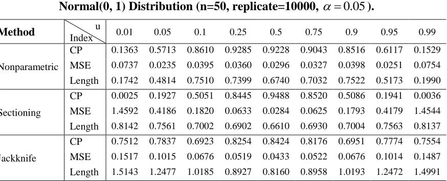
We choose sample size n50 in Tables 1-5. As seen in tables for u0.5, the sectioning approach has more CP than jackknife and nonparametric methods, but in some cases, MSE of this method is more than the two other methods and usually the length of CI of sectioning method is more than nonparametric approach. However for

0.1,0.25,0.75,0.9

u results of sectioning method is not satisfactory. In almost all distributions (except lognormal distribution for u0.9) CP of the nonparametric method is better than sectioning and jackknife methods, also MSE of this method is low and CI have the shortest length. Even in some cases for u0.05 or 0.95, the performance of the nonparametric method is better than the two other methods. As described in Section 2.2, in sectioning method, m should be relatively small and the number of observations k per section should be very large. When sample size is 50, with choosing m=10, the number of observations per section is equal to 5, where is very small, hence CI is violated in extreme quantiles. It should be noted that, as expressed in Section 2.3, we applied the jackknife approach to reducing the bias of sectioning method (where the simulation results show this), but the CP of sectioning method may be better than other approaches, as quantiles near the median.

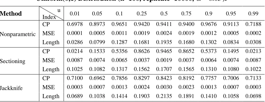
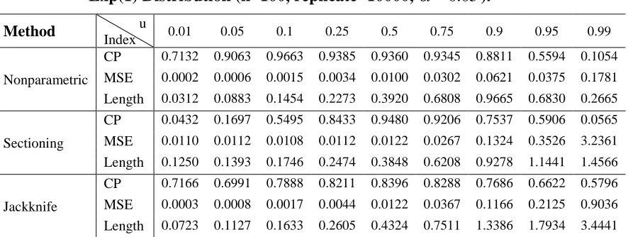
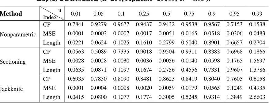
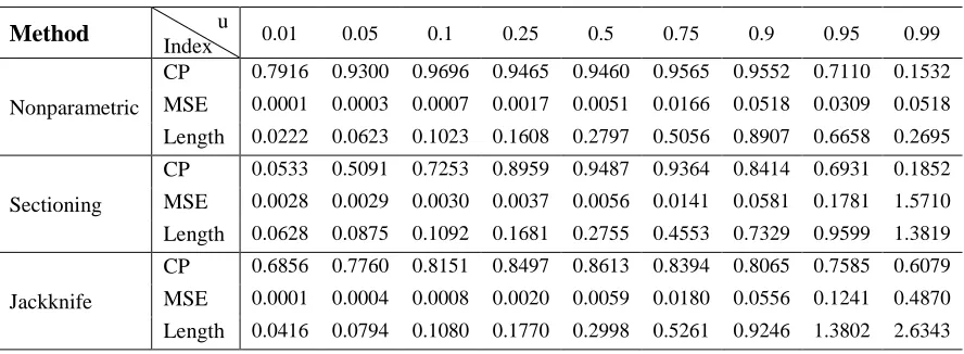
As the sample size increases to 100 (Tables 6-10) or 200 (Tables 11-15), results of nonparametric method improve in center and tails (especially in the lower tail), such that for u0.05,0.95 in most cases the nonparametric method outperforms the two other methods.

(8)

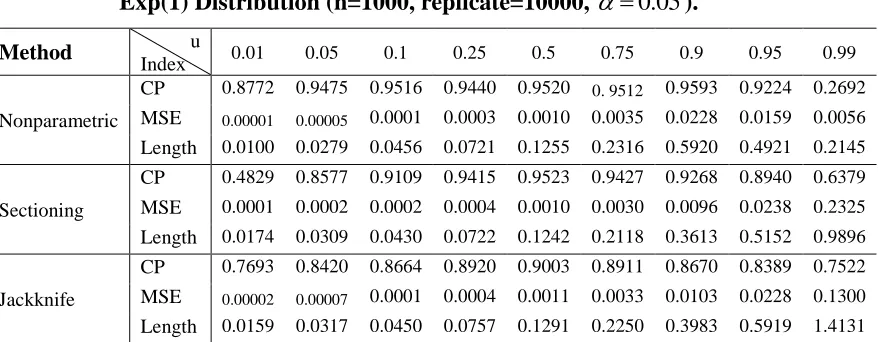
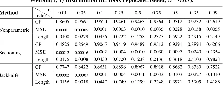
method has good results and in almost all cases CP, MSE and the expected length of CI in this method is better than sectioning and jackknife methods.

5. Conclusion

According to the simulation results, for small sample size, in estimation of CI for the median, sectioning method has better performance, and in tails the results of jackknife method is favorable. But for other quantiles, the nonparametric method has higher CP (in this work, close to 0.95), lower MSE and the shortest length in comparison with the two other methods. As the sample size increases, results of nonparametric method improve in center and tails (especially in the lower tail).

We emphasize that the results of nonparametric method have been achieved for constant bandwidth and we expect that the performance of this method increase by using optimal bandwidth.

Acknowledgments

The author would like to thank the reviewer for their valuable suggestions and comments.

References

1. Babu, G. J. (1986). Efficient estimation of the reciprocal of the density quantile function at a point. Statistics and Probability Letters, 4, 133-139.

2. Bloch, D. A. and Gastwirth, J. L. (1968). On a simple estimate of the reciprocal of the density function. Annals of Mathematical Statistics, 39, 1083-1085.

3. Bofinger, E. (1975). Estimation of a density function using order statistics. Australian Journal of Statistics, 17, 1-7.

4. Chesneau, C., Dewan, I. and Doosti, H. (2016). Nonparametric estimation of a quantile density function by wavelet methods. Computation Statistics and Data Analysis, 94, 161-174.

5. Falk, M. (1986). On the estimation of the quantile density function. Statistics and Probability Letters, 4, 69-73.

6. Jones, M. C. (1992). Estimating densities, quantiles, quantile densities and density quantiles. Annals of Institute of Statistical Mathematics, 44(4), 721-727.

7. Lewis, P. A. W. and Orav, J. (1988). Simulation Methodology for Statisticians, Operations Analysts, and Engineers, (Vol. 1). CRC press.

8. Nakayama, M. K. (2012). Confidence intervals for quantiles when applying replicated latin hypercube sampling and sectioning. Proceedings of the 2012 Autumn Simulation Conference, The Society for Modeling & Simulation International.

(9)

10. Parzen, E. (1979). Nonparametric statistical data modeling. Journal of the American Statistical Association, 7, 105-131.

11. Prakasa Rao, B. L. S. (1983). Nonparametric functional estimation. Academic Press.

12. R Core Team. (2014). R: A language and environment for statistical computing. R Foundation for Statistical Computing, Vienna, Austria. ISBN 3-900051-07-0, URL http://www.R-project.org/.

13. Reiss, R. D. (1978). Approximate distribution of the maximum deviation of histograms. Metrika, 25(1), 9-26.

14. Serfling, R. J. (1980). Approximation theorems of mathematical statistics. New York: Wiley.

15. Sheather, S. J. and Maritz, J. S. (1983). An estimate of the asymptotic standard error of the sample median. Australian Journal of Statistics, 25(1), 109-122.

16. Siddiqui, M. M. (1960). Distribution of quantitles in samples from a bivariate population. Journal of Research of the National Bureau of Standards, Section B, 64, 145-150.

17. Soni, P. and Dewan, I. and Jain, K. (2012). Nonparametric estimation of quantile density function. Computational Statistics and Data Analysis, 56, 3876-3886.

18. Steitnberg, S. M. (1983). Confidence intervals for functions of quantiles using linear combinations of order statistics. Ph. D. Thesis, University of North Carolina, Chapel Hill.

19. Tukey, J. W. (1965). Which part of the sample contains the information? Proceedings of the Mathemetical Academy of Science USA, 53, 127-134.

20. Wand, M. P. and Jones, M. C. (1995). Kernel smoothing; Monographs on statistics and applied probability. Chapman & Hall.

21. Welsh, A. H. (1988). Asymptotically efficient estimation of the sparsity function at a point. Statistics and Probability Letters, 6, 427-432.

(10)

Appendix

Table 1: CP, MSE and the length of CI for Various Choices of u in sampling from Uniform(0,1) Distribution (n=50, replicate=10000, 0.05).

Method _Indexu 0.01 0.05 0.1 0.25 0.5 0.75 0.9 0.95 0.99

Nonparametric

CP 0.6001 0.8722 0.9615 0.9346 0.9299 0.9252 0.9599 0.8963 0.6484

MSE 0.0005 0.0011 0.0024 0.0037 0.0048 0.0037 0.0025 0.0013 0.0005

Length 0.0393 0.1117 0.1818 0.2357 0.2707 0.2342 0.1855 0.1214 0.0455

Sectioning

CP 0.0085 0.0346 0.1735 0.7797 0.9475 0.7839 0.1663 0.0364 0.0081

MSE 0.0285 0.0245 0.0198 0.0103 0.0036 0.0102 0.0199 0.0243 0.0286

Length 0.1733 0.1714 0.1752 0.2206 0.2344 0.2207 0.1752 0.1714 0.1733

Jackknife

CP 0.8727 0.8119 0.6977 0.8201 0.8367 0.8231 0.7011 0.8127 0.8734

MSE 0.0007 0.0017 0.0026 0.0053 0.0067 0.0054 0.0026 0.0017 0.0007

Length 0.1026 0.1634 0.1979 0.2848 0.3212 0.2875 0.1981 0.1633 0.1032

Table 2: CP, MSE and the length of CI for Various Choices of u in sampling from Exp(1) Distribution (n=50, replicate=10000, 0.05).

Method u

Index 0.01 0.05 0.1 0.25 0.5 0.75 0.9 0.95 0.99

Nonparametric

CP 0.6289 0.8861 0.9611 0.9278 0.9175 0.8914 0.7374 0.4107 0.0736

MSE 0.0005 0.0014 0.0031 0.0069 0.0194 0.0475 0.0643 0.0483 0.3823

Length 0.0433 0.1242 0.2070 0.3187 0.5441 0.8534 0.9596 0.6436 0.2445

Sectioning

CP 0.0408 0.0611 0.1854 0.7739 0.9464 0.8672 0.6695 0.3160 0.0100

MSE 0.0441 0.0433 0.0430 0.0369 0.0298 0.0574 0.2584 0.9426 5.7174

Length 0.2490 0.2545 0.2776 0.3982 0.5743 0.8399 1.1305 1.3007 1.4608

Jackknife

CP 0.8779 0.8168 0.7269 0.8176 0.8417 0.8152 0.6784 0.7583 0.7210

MSE 0.0008 0.0022 0.0035 0.0100 0.0279 0.0851 0.2031 0.4013 0.9157

Length 0.1099 0.1827 0.2329 0.3928 0.6550 1.1432 1.7632 2.4787 3.7280

Table 3: CP, MSE and the length of CI for Various Choices of u in sampling from Normal(0, 1) Distribution (n=50, replicate=10000, 0.05).

Method u

Index 0.01 0.05 0.1 0.25 0.5 0.75 0.9 0.95 0.99

Nonparametric

CP 0.1363 0.5713 0.8610 0.9285 0.9228 0.9043 0.8516 0.6117 0.1529

MSE 0.0737 0.0235 0.0395 0.0360 0.0296 0.0327 0.0398 0.0251 0.0754

Length 0.1742 0.4814 0.7510 0.7399 0.6740 0.7032 0.7522 0.5173 0.1990

Sectioning

CP 0.0025 0.1927 0.5051 0.8445 0.9488 0.8520 0.5086 0.1941 0.0036

MSE 1.4592 0.4186 0.1820 0.0633 0.0284 0.0625 0.1793 0.4179 1.4544

Length 0.8142 0.7561 0.7002 0.6902 0.6610 0.6930 0.7004 0.7563 0.8137

Jackknife

CP 0.7512 0.7837 0.6923 0.8254 0.8424 0.8176 0.6951 0.7774 0.7554

MSE 0.1517 0.1015 0.0676 0.0519 0.0433 0.0522 0.0676 0.1014 0.1487

(11)

Table 4: CP, MSE and the length of CI for Various Choices of u in sampling from Lognormal(0, 1) Distribution (n=50, replicate=10000, 0.05).

Method _Indexu 0.01 0.05 0.1 0.25 0.5 0.75 0.9 0.95 0.99

Nonparametric

CP 0.4176 0.8382 0.9502 0.9335 0.9128 0.8479 0.4995 0.2100 0.0232

MSE 0.0021 0.0028 0.0059 0.0102 0.0298 0.0851 0.0969 0.0980 2.2224

Length 0.0650 0.1783 0.2867 0.3890 0.6740 1.1437 1.1757 0.7661 0.2825

Sectioning

CP 0.0151 0.0861 0.2559 0.7916 0.9405 0.8920 0.7781 0.4626 0.0464

MSE 0.0969 0.0733 0.0658 0.0580 0.0697 0.1469 0.7388 3.2679 40.377

Length 0.3252 0.3317 0.3601 0.5182 0.8320 1.4925 2.9955 3.7199 4.1655

Jackknife

CP 0.8249 0.8158 0.7215 0.8260 0.8363 0.8084 0.6654 0.7450 0.6716

MSE 0.0031 0.0052 0.0063 0.0152 0.0464 0.2122 0.9051 2.8640 15.912

Length 0.2166 0.2834 0.3116 0.4840 0.8441 1.8055 3.7060 6.6068 15.636

Table 5: CP, MSE and the length of CI for Various Choices of u in sampling from Weibull(1, 1) Distribution (n=50, replicate=10000, 0.05).

Method u

Index 0.01 0.05 0.1 0.25 0.5 0.75 0.9 0.95 0.99

Nonparametric

CP 0.6028 0.8849 0.9596 0.9306 0.9138 0.8894 0.7395 0.4113 0.0759

MSE 0.0005 0.0014 0.0032 0.0069 0.0194 0.0475 0.0639 0.0473 0.3659

Length 0.0432 0.1236 0.2070 0.3187 0.5426 0.8545 0.9569 0.6465 0.2445

Sectioning

CP 0.0369 0.0644 0.1785 0.7753 0.9457 0.8755 0.6686 0.3235 0.0104

MSE 0.0443 0.0436 0.0430 0.0367 0.0297 0.0572 0.2587 0.9404 5.7220

Length 0.2486 0.2557 0.2768 0.3960 0.5743 0.8448 1.1212 1.3101 1.4562

Jackknife

CP 0.8812 0.8107 0.7108 0.8203 0.8382 0.8122 0.6791 0.7611 0.7204

MSE 0.0008 0.0021 0.0035 0.0105 0.0283 0.0835 0.2019 0.4161 0.9365

Length 0.1092 0.1789 0.2318 0.4024 0.6589 1.1319 1.7579 2.5219 3.7683

Method _Indexu 0.01 0.05 0.1 0.25 0.5 0.75 0.9 0.95 0.99

Nonparametric

CP 0.6978 0.8973 0.9651 0.9420 0.9411 0.9400 0.9676 0.9113 0.7188

MSE 0.0001 0.0005 0.0011 0.0019 0.0024 0.0019 0.0012 0.0005 0.0002

Length 0.0286 0.0799 0.1287 0.1681 0.1935 0.1680 0.1302 0.0834 0.0308

Sectioning

CP 0.0214 0.1533 0.5356 0.8626 0.9465 0.8652 0.5373 0.1495 0.0213

MSE 0.0087 0.0074 0.0065 0.0037 0.0019 0.0037 0.0064 0.0074 0.0087

Length 0.1025 0.1082 0.1317 0.1562 0.1707 0.1565 0.1310 0.1080 0.1022

Jackknife

CP 0.7100 0.6962 0.7856 0.8297 0.8423 0.8192 0.7757 0.7006 0.7133

MSE 0.0003 0.0007 0.0013 0.0024 0.0030 0.0023 0.0013 0.0007 0.0003

(12)

Method _Indexu 0.01 0.05 0.1 0.25 0.5 0.75 0.9 0.95 0.99

Nonparametric

CP 0.7132 0.9063 0.9663 0.9385 0.9360 0.9345 0.8811 0.5594 0.1054

MSE 0.0002 0.0006 0.0015 0.0034 0.0100 0.0302 0.0621 0.0375 0.1781

Length 0.0312 0.0883 0.1454 0.2273 0.3920 0.6808 0.9665 0.6830 0.2665

Sectioning

CP 0.0432 0.1697 0.5495 0.8433 0.9480 0.9206 0.7537 0.5906 0.0565

MSE 0.0110 0.0112 0.0108 0.0112 0.0122 0.0267 0.1324 0.3526 3.2361

Length 0.1250 0.1393 0.1746 0.2474 0.3848 0.6208 0.9278 1.1441 1.4566

Jackknife

CP 0.7166 0.6991 0.7888 0.8211 0.8396 0.8288 0.7686 0.6622 0.5796

MSE 0.0003 0.0008 0.0017 0.0044 0.0122 0.0367 0.1166 0.2125 0.9036

Length 0.0723 0.1127 0.1633 0.2605 0.4324 0.7511 1.3386 1.7934 3.4441

Method u

Index 0.01 0.05 0.1 0.25 0.5 0.75 0.9 0.95 0.99

Nonparametric

CP 0.1931 0.7234 0.9467 0.9459 0.9389 0.9359 0.9456 0.7459 0.1990

MSE 0.0314 0.0171 0.0313 0.0197 0.0156 0.0188 0.0304 0.0175 0.0316

Length 0.1832 0.4759 0.6852 0.5491 0.4901 0.5362 0.6771 0.4869 0.1938

Sectioning

CP 0.0267 0.4620 0.6929 0.8990 0.9516 0.8941 0.6900 0.4715 0.0269

MSE 0.7267 0.1443 0.0716 0.0233 0.0139 0.0240 0.0723 0.1432 0.7364

Length 0.6964 0.5965 0.5639 0.4938 0.4622 0.4928 0.5658 0.5975 0.6950

Jackknife

CP 0.6095 0.6743 0.7860 0.8206 0.8462 0.8296 0.7783 0.6739 0.6075

MSE 0.1318 0.0507 0.0384 0.0233 0.0189 0.0233 0.0387 0.0507 0.1323

Length 1.3467 0.8804 0.7679 0.5983 0.5388 0.5977 0.7710 0.8814 1.3560

Method _Indexu 0.01 0.05 0.1 0.25 0.5 0.75 0.9 0.95 0.99

Nonparametric

CP 0.4481 0.8672 0.9640 0.9430 0.9393 0.9251 0.7201 0.3229 0.0340

MSE 0.0007 0.0013 0.0029 0.0051 0.0161 0.0672 0.1182 0.0770 1.3345

Length 0.0487 0.1319 0.2055 0.2791 0.4960 1.0163 1.3342 0.9051 0.3417

Sectioning

CP 0.0130 0.2511 0.5834 0.8466 0.9427 0.9278 0.8257 0.7261 0.1317

MSE 0.0303 0.0187 0.0167 0.0165 0.0251 0.0714 0.3698 1.2822 25.193

Length 0.1764 0.1861 0.2233 0.3065 0.5189 1.0470 2.0936 3.4594 4.8413

Jackknife

CP 0.6684 0.6947 0.7828 0.8271 0.8484 0.8163 0.7629 0.6519 0.5288

MSE 0.0019 0.0022 0.0032 0.0063 0.0195 0.0904 0.5000 1.3808 15.718

(13)

Method _Indexu 0.01 0.05 0.1 0.25 0.5 0.75 0.9 0.95 0.99

Nonparametric

CP 0.7238 0.9156 0.9667 0.9366 0.9317 0.9345 0.8849 0.5541 0.1071

MSE 0.0002 0.0006 0.0015 0.0034 0.0100 0.0304 0.0620 0.0382 0.1737

Length 0.0311 0.0880 0.1451 0.2267 0.3919 0.6831 0.9677 0.6820 0.2667

Sectioning

CP 0.0427 0.1712 0.5345 0.8410 0.9431 0.9210 0.7503 0.5819 0.0524

MSE 0.0111 0.0110 0.0110 0.0109 0.0124 0.0266 0.1306 0.3535 3.2660

Length 0.1256 0.1388 0.1749 0.2453 0.3844 0.6202 0.9276 1.1349 1.4512

Jackknife

CP 0.7219 0.7029 0.7855 0.8276 0.8419 0.8314 0.7781 0.6688 0.5788

MSE 0.0003 0.0008 0.0017 0.0044 0.0122 0.0375 0.1195 0.2124 0.8850

Length 0.0725 0.1119 0.1629 0.2586 0.4321 0.7587 1.3552 1.8002 3.4177

Method u

Index 0.01 0.05 0.1 0.25 0.5 0.75 0.9 0.95 0.99

Nonparametric

CP 0.7691 0.9174 0.9629 0.9469 0.9427 0.9433 0.9670 0.9225 0.7738

MSE 0.0001 0.0002 0.0006 0.0009 0.0012 0.0009 0.0006 0.0002 0.0001

Length 0.0204 0.0567 0.0908 0.1198 0.1378 0.1197 0.0914 0.0580 0.0212

Sectioning

CP 0.0431 0.5081 0.7378 0.9086 0.9505 0.9101 0.7288 0.5051 0.0404

MSE 0.0024 0.0022 0.0020 0.0014 0.0011 0.0014 0.0020 0.0022 0.0024

Length 0.0567 0.0761 0.0895 0.1150 0.1287 0.1153 0.0897 0.0752 0.0565

Jackknife

CP 0.6870 0.7797 0.8103 0.8434 0.8603 0.8489 0.8080 0.7736 0.6927

MSE 0.0001 0.0004 0.0006 0.0011 0.0015 0.0011 0.0006 0.0004 0.0001

Length 0.0405 0.0748 0.0969 0.1306 0.1494 0.1316 0.0960 0.0746 0.0407

Method _Indexu 0.01 0.05 0.1 0.25 0.5 0.75 0.9 0.95 0.99

Nonparametric

CP 0.7841 0.9279 0.9677 0.9437 0.9432 0.9538 0.9567 0.7153 0.1538

MSE 0.0001 0.0003 0.0007 0.0017 0.0051 0.0165 0.0518 0.0306 0.0483

Length 0.0221 0.0624 0.1025 0.1610 0.2799 0.5040 0.8901 0.6657 0.2704

Sectioning

CP 0.0563 0.5089 0.7335 0.9018 0.9504 0.9311 0.8383 0.6968 0.1866

MSE 0.0028 0.0028 0.0030 0.0036 0.0056 0.0140 0.0598 0.1765 1.5697

Length 0.0635 0.0871 0.1097 0.1674 0.2756 0.4556 0.7331 0.9607 1.3786

Jackknife

CP 0.6935 0.7830 0.8090 0.8481 0.8623 0.8419 0.8040 0.7605 0.6058

MSE 0.0001 0.0004 0.0008 0.0020 0.0059 0.0179 0.0565 0.1249 0.4935

(14)

Method _Indexu 0.01 0.05 0.1 0.25 0.5 0.75 0.9 0.95 0.99

Nonparametric

CP 0.2469 0.8218 0.9769 0.9557 0.9489 0.9470 0.9744 0.8370 0.2569

MSE 0.0106 0.0122 0.0212 0.0101 0.0080 0.0099 0.0208 0.0123 0.0109

Length 0.1698 0.4207 0.5682 0.3943 0.3513 0.3889 0.5621 0.4238 0.1736

Sectioning

CP 0.1297 0.6518 0.8187 0.9249 0.9502 0.9218 0.8150 0.6478 0.1309

MSE 0.3218 0.0612 0.0268 0.0108 0.0073 0.0106 0.0270 0.0616 0.3229

Length 0.5915 0.4935 0.4310 0.3626 0.3358 0.3615 0.4310 0.4911 0.5924

Jackknife

CP 0.6171 0.7737 0.8124 0.8425 0.8651 0.8498 0.8025 0.7601 0.6186

MSE 0.0722 0.0294 0.0187 0.0110 0.0091 0.0110 0.0184 0.0296 0.0722

Length 1.0251 0.6725 0.5353 0.4119 0.3739 0.4113 0.5323 0.6746 1.0321

Method u

Index 0.01 0.05 0.1 0.25 0.5 0.75 0.9 0.95 0.99

Nonparametric

CP 0.4892 0.8930 0.9690 0.9447 0.9438 0.9511 0.8857 0.4900 0.0613

MSE 0.0002 0.0006 0.0014 0.0026 0.0082 0.0409 0.1262 0.0687 0.4003

Length 0.0350 0.0944 0.1462 0.1976 0.3541 0.7921 1.3900 1.0015 0.3919

Sectioning

CP 0.0432 0.5612 0.7638 0.9041 0.9435 0.9391 0.8636 0.7529 0.3159

MSE 0.0097 0.0055 0.0046 0.0051 0.0102 0.0353 0.1971 0.7507 12.566

Length 0.1055 0.1266 0.1435 0.2036 0.3571 0.7360 1.5649 2.5280 5.3603

Jackknife

CP 0.6639 0.7805 0.8098 0.8478 0.8647 0.8479 0.8054 0.7549 0.5813

MSE 0.0009 0.0012 0.0015 0.0029 0.0093 0.0436 0.2461 0.7921 8.0904

Length 0.1155 0.1358 0.1508 0.2110 0.3776 0.8188 1.9445 3.4881 10.635

Method _Indexu 0.01 0.05 0.1 0.25 0.5 0.75 0.9 0.95 0.99

Nonparametric

CP 0.7916 0.9300 0.9696 0.9465 0.9460 0.9565 0.9552 0.7110 0.1532

MSE 0.0001 0.0003 0.0007 0.0017 0.0051 0.0166 0.0518 0.0309 0.0518

Length 0.0222 0.0623 0.1023 0.1608 0.2797 0.5056 0.8907 0.6658 0.2695

Sectioning

CP 0.0533 0.5091 0.7253 0.8959 0.9487 0.9364 0.8414 0.6931 0.1852

MSE 0.0028 0.0029 0.0030 0.0037 0.0056 0.0141 0.0581 0.1781 1.5710

Length 0.0628 0.0875 0.1092 0.1681 0.2755 0.4553 0.7329 0.9599 1.3819

Jackknife

CP 0.6856 0.7760 0.8151 0.8497 0.8613 0.8394 0.8065 0.7585 0.6079

MSE 0.0001 0.0004 0.0008 0.0020 0.0059 0.0180 0.0556 0.1241 0.4870

(15)

Method _Indexu 0.01 0.05 0.1 0.25 0.5 0.75 0.9 0.95 0.99

Nonparametric

CP _{0.8327 0.9319 0.9681 0.9534 0.9420 0.9405 0.9744 0.9421 0.8543}

MSE 0.00001 0.00004 0.0001 0.0002 0.0002 0.0002 0.0001 0.00004 0.00001

Length 0.0092 0.0255 0.0405 0.0536 0.0619 0.0538 0.0407 0.0256 0.0093

Sectioning

CP _{0.4786 0.8532 0.9117 0.9391 0.9489 0.9439 0.9094 0.8532 0.4839}

MSE 0.00011 0.00013 0.0002 0.0002 0.0002 0.0002 0.0002 0.00013 0.00011

Length 0.0170 0.0288 0.0379 0.0531 0.0610 0.0533 0.0379 0.0288 0.0169

Jackknife

CP _{0.7693 0.8444 0.8685 0.8951 0.8993 0.8942 0.8614 0.8443 0.7751}

MSE 0.00002 0.00006 0.0001 0.0002 0.0003 0.0002 0.0001 0.00006 0.00002

Length _{0.0155 0.0299 0.0404 0.0565 0.0644 0.0564 0.0400 0.0301 0.0156}

Method u

Index 0.01 0.05 0.1 0.25 0.5 0.75 0.9 0.95 0.99

Nonparametric

CP 0.8772 0.9475 0.9516 0.9440 0.9520 0. 9512 0.9593 0.9224 0.2692

MSE 0.00001 0.00005 0.0001 0.0003 0.0010 0.0035 0.0228 0.0159 0.0056

Length 0.0100 0.0279 0.0456 0.0721 0.1255 0.2316 0.5920 0.4921 0.2145

Sectioning

CP 0.4829 0.8577 0.9109 0.9415 0.9523 0.9427 0.9268 0.8940 0.6379

MSE 0.0001 0.0002 0.0002 0.0004 0.0010 0.0030 0.0096 0.0238 0.2325

Length 0.0174 0.0309 0.0430 0.0722 0.1242 0.2118 0.3613 0.5152 0.9896

Jackknife

CP 0.7693 0.8420 0.8664 0.8920 0.9003 0.8911 0.8670 0.8389 0.7522

MSE 0.00002 0.00007 0.0001 0.0004 0.0011 0.0033 0.0103 0.0228 0.1300

Length 0.0159 0.0317 0.0450 0.0757 0.1291 0.2250 0.3983 0.5919 1.4131

Method _Indexu 0.01 0.05 0.1 0.25 0.5 0.75 0.9 0.95 0.99

Nonparametric

CP 0.3791 0.9437 0.9597 0.9519 0.9520 0.9617 0.9428 0.9474 0.3783

MSE 0.0011 0.0044 0.0066 0.0020 0.0016 0.0020 0.0066 0.0044 0.0010

Length 0.1120 0.2592 0.3194 0.1774 0.1576 0.1769 0.3183 0.2603 0.1117

Sectioning

CP 0.6065 0.8784 0.9237 0.9472 0.9474 0.9457 0.9219 0.8882 0.6155

MSE 0.0403 0.0065 0.0035 0.0019 0.0016 0.0019 0.0035 0.0066 0.0402

Length 0.3827 0.2512 0.2080 0.1671 0.1543 0.1677 0.2081 0.2521 0.3842

Jackknife

CP 0.7580 0.8420 0.8645 0.8838 0.9054 0.8910 0.8682 0.8405 0.7593

MSE 0.0187 0.0052 0.0033 0.0021 0.0017 0.0021 0.0034 0.0054 0.0187

(16)

Method _Indexu 0.01 0.05 0.1 0.25 0.5 0.75 0.9 0.95 0.99

Nonparametric

CP 0.5124 0.8903 0.9547 0.9582 0.9601 0.9518 0.9417 0.8451 0.1840

MSE 0.00002 0.0001 0.0003 0.0005 0.0017 0.0090 0.0894 0.0613 0.0422

Length 0.0159 0.0426 0.0655 0.0884 0.1595 0.3716 1.1719 0.9685 0.4159

Sectioning

CP 0.5597 0.8691 0.9206 0.9413 0.9541 0.9428 0.9299 0.9003 0.6887

MSE 0.0007 0.0004 0.0004 0.0006 0.0017 0.0071 0.0384 0.1317 2.3786

Length 0.0448 0.0516 0.0596 0.0872 0.1564 0.3309 0.7473 1.3006 3.8243

Jackknife

CP 0.7645 0.8459 0.8698 0.8951 0.9002 0.8885 0.8661 0.8397 0.7488

MSE 0.0002 0.0002 0.0003 0.0005 0.0017 0.0079 0.0436 0.1451 1.9471

Length 0.0537 0.0560 0.0636 0.0903 0.1625 0.3490 0.8183 1.4929 5.4697

Method u

Index 0.01 0.05 0.1 0.25 0.5 0.75 0.9 0.95 0.99

Nonparametric

CP 0.8605 0.9561 0.9520 0.9461 0.9463 0.9564 0.9512 0.9232 0.2619

MSE 0.00001 0.00005 0.0001 0.0003 0.0010 0.0035 0.0228 0.0158 0.0055

Length 0.0100 0.0279 0.0456 0.0722 0.1258 0.2327 0.5922 0.4915 0.2149

Sectioning

CP 0.4825 0.8549 0.9065 0.9419 0.9489 0.9512 0.9291 0.8894 0.6206

MSE 0.00012 0.00016 0.0002 0.0004 0.0010 0.0030 0.0097 0.0240 0.2354

Length 0.0175 0.0308 0.0430 0.0720 0.1238 0.2136 0.3618 0.5103 0.9828

Jackknife

CP 0.7747 0.8422 0.8631 0.8898 0.8967 0.8918 0.8662 0.8380 0.7522

MSE 0.00002 0.00007 0.0001 0.0004 0.0011 0.0033 0.0103 0.0227 0.1310