Warm winter, thin ice?

© Author(s) 2018. This work is distributed under the Creative Commons Attribution 4.0 License.

Warm winter, thin ice?

Julienne C. Stroeve1,2, David Schroder3, Michel Tsamados1, and Daniel Feltham3

1_{Centre for Polar Observation and Modelling, Earth Sciences, University College London, London, UK} 2_{National Snow and Ice Data Center, University of Colorado, Boulder, CO, USA}

3_{Centre for Polar Observation and Modelling, Department of Meteorology, University of Reading, Reading, UK} Correspondence:Julienne C. Stroeve ([email protected])

Received: 29 December 2017 – Discussion started: 11 January 2018 Revised: 9 April 2018 – Accepted: 10 April 2018 – Published: 30 May 2018

Abstract. Winter 2016/2017 saw record warmth over the Arctic Ocean, leading to the least amount of freezing de-gree days north of 70◦N since at least 1979. The impact of this warmth was evaluated using model simulations from the Los Alamos sea ice model (CICE) and CryoSat-2 thickness estimates from three different data providers. While CICE simulations show a broad region of anomalously thin ice in April 2017 relative to the 2011–2017 mean, analysis of three CryoSat-2 products show more limited regions with thin ice and do not always agree with each other, both in magnitude and direction of thickness anomalies. CICE is further used to diagnose feedback processes driving the observed anomalies, showing 11–13 cm reduced thermodynamic ice growth over the Arctic domain used in this study compared to the 2011– 2017 mean, and dynamical contributions of +1 to+4 cm. Finally, CICE model simulations from 1985 to 2017 indicate the negative feedback relationship between ice growth and winter air temperatures may be starting to weaken, showing decreased winter ice growth since 2012, as winter air tem-peratures have increased and the freeze-up has been further delayed.

1 Introduction

It is well known that Arctic air temperatures are rising faster than the global average (e.g., Bekryaev et al., 2010; Serreze and Barry, 2011). The thinning and shrinking of the sum-mer sea ice cover have played a role in this amplified warm-ing, which is most prominent during the autumn and winter months, as the heat gained by the ocean mixed layer during ice-free summer periods is released back to the atmosphere during ice formation (e.g. Serreze et al., 2009; Screen and

Simmonds, 2010). However, Arctic amplification has been found in climate models without changes in the sea ice cover (Pithan and Mauritsen, 2014). Increased latent energy trans-port (Graversen and Burtu, 2016), the lapse rate feedback (Pithan and Mauritsen, 2014; Graversen, 2006) and changes in ocean circulation (Polyakov et al., 2005) have also con-tributed. Furthermore, cyclones are effective means of bring-ing warm and moist air into the Arctic durbring-ing winter (e.g., Boisvert et al., 2016).

Winter 2015/2016 was previously reported as the warmest Arctic winter recorded since records began in 1950 (Cul-lather et al., 2016). Warming was Arctic-wide, with temper-ature anomalies reaching+5◦C (Overland and Wang, 2016) and temperatures near the North Pole hitting 0◦_{C (Boisvert} et al., 2016). Part of the unusual warming was linked to a strong cyclone that entered the Arctic in December 2015 (Boisvert et al., 2016), resulting in reduced thermodynamic ice growth and thinning within the Kara and Barents seas (Ricker et al., 2017a; Boisvert et al., 2016). This was one of several cyclones to enter the Arctic that winter as a result of a split tropospheric vortex that brought warm and moist air from the Atlantic Ocean towards the pole (Overland and Wang, 2016). Winter 2016/2017 once again saw tempera-tures near the North Pole reach 0◦C in December 2016 and February 2017 (Graham et al., 2017). These warming events were similarly associated with large storms entering the Arc-tic (Cohen et al., 2017). It has been suggested that the re-cent warm winters represent a trend towards increased dura-tion and intensity of winter warming events within the central Arctic (Graham et al., 2017).

the period for snow accumulation on the sea ice. Stroeve et al. (2014) previously evaluated changes in the melt on-set and freeze-up, showing large delays in freeze-up within the Chukchi, East Siberian, Laptev and Barents seas, with delays increasing in the order of+10 days per decade. Later freeze-up has a non-trivial influence on basin-wide sea ice thickness: ice grows thermodynamically faster for thin ice than for thick ice (Bitz and Roe, 2004). More subtle effects involving the timing of ice growth relative to major snow pre-cipitation events in fall have been shown to also control the growth rate of sea ice thickness; ice grows faster for a thinner snow pack (Merkouriadi et al., 2017). Nevertheless, the max-imum winter sea ice extent in 2017 set a new record low for the 3rd year in a row. Have the recent warm winters played a role in these record low winter maxima by reducing winter ice formation?

Ricker et al. (2017a) previously evaluated the impact of the 2015/2016 warm winter on ice growth using sea ice thick-ness derived from blending CryoSat-2 (CS2) radar altimetry with those from Soil Moisture and Ocean Salinity (SMOS) radiometry (Ricker et al., 2017b). They found anomalous freezing degree days (FDDs) between November 2015 and March 2016 within the Barents Sea of 1000◦ days coin-cided with a thinning of approximately 10 cm in March com-pared to the 6-year mean. While near-surface air tempera-tures largely control thermodynamic ice growth, other pro-cesses also impact ice growth, including ocean circulation, sensible and latent heat exchanges. Furthermore, winter ice thickness is not only a result of thermodynamic ice growth, but rather the combined effects of thermodynamic and dy-namic processes. A thinner ice cover is more prone to ridging and rafting, as well as ice divergence, leading to new ice for-mation within leads and cracks within the ice pack. However, this was not evaluated by Ricker et al. (2017a).

In this study we evaluate the impact of the 2016/2017 anomalously warm winter on Arctic sea ice thickness us-ing the Los Alamos sea ice model (CICE) (Hunke et al., 2015) and satellite-derived CS2 thickness data from three different sources: Centre for Polar Observation and Mod-eling (CPOM) (Tilling et al., 2017), Alfred Wegener Insti-tute (AWI) (Hendricks et al., 2016) and NASA (Kurtz and Harbeck, 2017). CICE is initialized with CPOM CS2 sub-grid scale ice thickness distribution (ITD) fields in Novem-ber and run forward with NCEP Reanalysis-2 (NCEP2) at-mospheric reanalysis data (Kanamitsu et al., 2002, updated 2017). The model run is subsequently compared over the winter growth season to CS2 thickness from the three differ-ent data providers and contributions of thermodynamics vs. dynamics to the thickness anomalies are evaluated. While the focus is on the 2016/2017 ice growth season, a secondary aim is to compare existing CS2 products to inform the commu-nity on uncertainties in these estimates and inform on model limitations. Thus, results are also presented for other years during the CS2 time-period for comparison. To our

knowl-edge, this is the first study to compare different CS2 data products over the lifetime of the mission.

2 Methods

2.1 Ice thickness distribution (ITD) from Cryosat-2

The CryoSat-2 radar altimetry mission was launched April 2010, providing estimates of ice thickness during the ice growth season. CS2 provides freeboard estimates, or the height of the ice surface above the local sea surface, which when combined with information on snow depth, snow den-sity and ice denden-sity can be converted to ice thickness assum-ing hydrostatic equilibrium (e.g., Laxon et al., 2013). Here we evaluate ice thickness fields provided by three different data providers in order to assess robustness of the observed thickness anomalies. Thickness is retrieved from ice free-board by processing CS2 Level 1B data, with a footprint of 300 m by 1700 m, and assuming snow density and snow depth from the Warren et al. (1999) climatology (hereafter W99), modified for the distribution of multi-year vs. first-year ice (i.e., snow depth is halved over first-first-year ice) (see Laxon et al., 2013 and Tilling et al., 2017 for data processing details).

While the three data providers rely on W99 for snow depth and density, each institution processes the radar returns dif-ferently. In general, the range to the main scattering hori-zon of the radar return is obtained using a retracker algo-rithm. This can be based on a threshold (e.g Laxon et al., 2013; Ricker et al., 2014; Hendricks et al., 2016) or a phys-ical retracker (Kurtz et al., 2014). While the CPOM and AWI products use a leading edge 70 % threshold retracker, Kurtz and Harbeck (2017) rely on a physical model to best fit each CryoSat-2 waveform. This will lead to ice thickness differences based on different thresholds applied: Kurtz et al. (2014) found a 12 cm mean difference between using a 50 % threshold and a waveform fitting method.

We note that several factors contribute to CS2-derived sea ice thickness uncertainties, including the assumption that the radar return is from the snow or ice interface (Willat et al., 2011), snow depth departures from climatology and the use of fixed snow and ice densities. In this study we initialize the CICE model simulations described below with the CPOM sea ice thickness fields. Accuracy of the CPOM product has been evaluated in several studies, suggesting mean biases be-tween thickness observations in 2011 and 2012 of 6.6 cm, when compared with airborne EM data (Laxon et al., 2013; Tilling et al., 2015). For April 2017, the CPOM near-real-time product (Tilling et al., 2016) was used in place of the archived product, with a mean thickness bias of 0.9 cm be-tween these products.

rectangu-lar 50 km grid for each month. The mean area fraction and mean thickness is derived for each thickness category and these values are interpolated on the tripolar 1◦ _{CICE grid} (∼40 km grid resolution). Grid points with less than 100 in-dividual measurements and a mean SIT <0.5 m are not in-cluded. Otherwise, all individual observations are inin-cluded. For November, this effectively limits the area of the Arctic to the region shown in Fig. 1c. Negative thickness values that are retained in the CS2 processing to prevent statistical posi-tive bias of the thinner ice are added to category 1. The novel approach of initializing the CICE model with the full ITD rather than the mean sea ice thickness provides an additional control on the repartition of the ice among different thickness categories. This in turn allows a more accurate representa-tion of ice growth and ice melt processes (Tsamados et al., 2015) compared to initializing with the mean grid-cell SIT and deriving the fractions for each ice category assuming a parabolic distribution. Ice growth and melt strongly depend on SIT: using a real distribution can have a big impact, espe-cially for thin ice.

2.2 CICE simulations

CICE is a dynamic thermodynamic sea ice model designed for inclusion within a global climate model. The advantages of using CICE for this study is that we can more readily sep-arate thickness anomalies into their thermodynamic and dy-namical contributions, examine inter-annual variability and perform longer simulations. For this study, we performed two different CICE simulations. The first is a multi-year simula-tion from 1985 to 2017 (referred to as CICE-free). The sec-ond is a stand-alone sea ice simulation for the pan-Arctic region starting in mid-November and running until the end of April of the following year for the last seven winter pe-riods from 2010/2011 to 2016/2017. This results in seven 1-year long simulations (referred to as CICE-ini), in which the initial thickness and concentration for each of the five ice categories is updated from the CS2 ITD using the CPOM CS2 November thickness fields. For grid points without CS2 data, and for all other variables (e.g., temperature profiles, snow volume), results from the free CICE simulation with the same configuration, started in 1985, are applied. In this way, CICE simulations cover the pan-Arctic region, but in regions where no CS2 are available, we restart SIT values from the free CICE model run. While this approach would be problematic in a coupled model, in a stand-alone sea ice sim-ulation the model adjustment to the new conditions is smooth and the impact of using the vertical temperature profile from the free simulation only affects sea ice thickness in the order of millimeters.

Snow accumulation can depart strongly from the W99 cli-matology for individual years. Thus, we make the assump-tion that the deviaassump-tion of the mean annual cycle of snow depth over the last 7 years from the W99 climatology is small and assume mean winter ice growth to be determined

accu-rately from CS2, and tuned CICE-ini accordingly to match the observed CS2 mean winter ice growth from the CPOM product in the central Arctic (Fig. 1). The excellent agree-ment for both CICE-ini and CICE-free with CS2 increases the confidence of our model results. Therefore, our approach allows us to study inter-annual variability from two model configurations with different sources of errors, in addition to the three CS2-based products.

For both CICE simulations, NCEP-2 provides the atmo-spheric forcing. We use NCEP-2 2 m air temperatures be-cause they have been shown to be more realistic for the Arctic Ocean than those from ERA-Interim (Jakobshavn et al., 2012). The setup is the same as described in Schröder et al. (2014), including a simple ocean-mixed layer model, a prognostic melt pond model (Flocco et al., 2012) and an elastic anisotropic-plastic rheology (Tsamados et al., 2013), with the following improvements: we apply an updated CICE version 5.1.2 with variable atmospheric and oceanic form drag parameterization (Tsamados et al., 2014), we in-crease the thermal conductivity of fresh ice from 2.03 to 2.63 W m−1K−1, snow from 0.3 to 0.5 W m−1K−1and the emissivity of snow and ice from 0.95 to 0.976. While the de-fault conductivity values are at the lower end of the observed range, the new values are at the upper end and have been ap-plied in previous climate simulations (e.g., Rae et al., 2014). Below, all CS2-derived sea ice thickness anomalies are computed relative to the CS2 time-period: November anoma-lies are relative to 2010–2016 and for April they are rela-tive to 2011–2017. Results for November and April are only shown for all grid cells that have a minimum thickness of 50 cm and a minimum of 100 individual measurements for each of the seven years. For the month of November, this cor-responds to all colored areas shown in Fig. 1c. For April, this region represents the area in red shown in Fig. 1d. The larger region shown in Fig. 1d also corresponds to the region over which the amount of thermodynamic ice growth and dynam-ical ice growth between November and April are assessed from the CICE simulations. For comparison with CS2, we present the mean thickness of the ice-covered area. In winter, the sea ice concentration in the model generally ranges be-tween 0.98 and 0.995 % apart from locations close to the ice edge. Further note that area-averaged values for November and April are only given for regions shown in Fig. 1c and d, respectively.

3 Results

3.1 Air temperature and freezing anomalies

Figure 1.Comparison of CPOM CryoSat-2 mean seasonal sea ice thickness (black) with CICE free (blue) and CICE initialized with Cryosat-2 in November (red). Panel (a)shows results for mean thickness, averaged over all the colored areas shown in panel(c), representing the total region for which Cryosat-2 data exist in November (only grid points included with>100 measurements per month and mean thickness>0.5 m) and(b)mean thickness averaged over the sub-region shown in blue with medium thick ice in January (between 1.5 and 2.5 m). Blue areas in panel(c)show regions between November and January where CryoSat-2 thickness are between 1.5 and 2.5 m in all years; red for thin ice (<1.5) and orange for thick ice (>2.5 m). Panel(d)is the region over which the April thickness anomalies and results are presented.

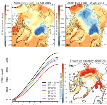
Ricker et al. (2017a). FDDs computed this way reflect both the number of days with air temperatures below freezing and the magnitude of below freezing air temperatures over the specified period. Spatially, FDD anomalies show widespread reductions over most of the Arctic Ocean, with the largest reductions in the Barents and Kara seas, stretching across the pole towards the Beaufort and Chukchi seas (Fig. 2b). In contrast, during winter 2015/2016, FDDs were most no-tably anomalous within the Barents and Kara seas (Fig. 2a), in agreement with Ricker et al. (2017a). Overall, as averaged from 70–90◦N, winter 2016/2017 witnessed the least amount of cumulative FDDs since at least 1979 (Fig. 2c).

While ice forms quickly within the central Arctic once air temperatures drop below freezing, 2016/2017 saw large de-lays in freeze-up throughout the Arctic. Updating results pre-viously reported in Stroeve et al. (2014), freeze-up was

de-layed by 20 days for the Arctic as a whole, with regions like the Bering, Beaufort, Chukchi, East Siberian and Kara seas delayed by 3 to 4 weeks (Fig. 2d). Within the Barents Sea, the regionally averaged freeze-up was delayed by 60 days. In recent years, the trend towards later freeze-up has increased, with the Barents and Chukchi seas showing the largest trends in the order of+14 days per decade through 2017, followed by the Kara and East Siberian seas with delays in the order of +10 to +12 days per decade. Within the Beaufort Sea, freeze-up is now happening later by+9 days per decade (Ta-ble 1).

3.2 November ice thickness anomalies

Figure 2.The top two panels show the freezing degree anomalies (FDD), computed as the number of days with NCEP2 2 m air temperature below−1.8◦C from mid-November to mid-April in winter 2016(a), and winter 2017(b), computed relative to the 1981–2010 climatology. The bottom left image shows the cumulative freezing degree days (FDDs) averaged over region shown in Fig. 3 inset(c), and the bottom right image shows freeze-up anomalies for 2016/2017 relative to 1981–2010(d). Areas in white are either missing (pole hole) or no sea ice in winter 2016/2017.

useful to first intercompare the different CryoSat-2 thickness estimates. We start with a comparison of November thick-ness from the three CS2 data sets from November 2010 to 2016 (Fig. 3). It is encouraging to find that year-to-year vari-ability in the spatial patterns of positive and negative thick-ness anomalies are generally consistent between the three products despite differences in waveform processing. The AWI and CPOM data sets are in better agreement with each other than with the NASA product, which is expected as they use a similar retracker. Furthermore, all three data sets show widespread thinner ice in November 2011, and widespread thicker ice in November 2013. This is further supported by analysis of regional mean thickness and anomalies computed over the region shown in Fig. 1c (Table 2). For comparison, we also list results from the CICE-free model simulation. In November 2011, the different CS2 data products are in agree-ment that the ice was anomalously thin (−32 to −46 cm), the thinnest in the CS2 data record. Similarly, in

Novem-ber 2013, all three CS2 products show overall thicker ice in the order of+23 to+38 cm. The CICE-free simulations also show anomalously thinner and thicker ice during these years, but larger anomalies were simulated in 2012 and 2014.

Table 1.Regional trends in freeze-up, 2017 freeze-up date and anomaly (relative to 1981–2010 mean). Freeze-up is computed following Markus et al. (2009).

Region Freeze-up trend 2017 mean freeze-up 2017 freeze-up (days per decade) (day of year) Anomaly (days)

Sea of Okhotsk 9.1 304 0.8

Bering Sea 6.7 338 25.2

Hudson Bay 7.9 333 16.9

Baffin Bay 8.0 312 13.2

E. Greenland Sea 5.6 267 2.7

Barents Sea 13.6 347 60.3

Kara Sea 10.7 314 36.6

Laptev Sea 9.0 272 10.7

E. Siberian Sea 11.8 286 27.1

Chukchi Sea 14.1 314 31.0

Beaufort Sea 8.9 279 23.4

Canadian Archipelago 4.9 268 12.7

Central Arctic 3.1 255 16.8

Pan-Arctic 7.5 288 19.6

Table 2.Mean November ice thickness and anomaly with respect to the 2011–2017 mean (in parentheses) from CS2 derived from CPOM, AWI and NASA. Spatial mean is over the Arctic Basin, defined as the area for which CS-data were available continuously for all seven winter periods November to April 2010/2011 to 2016/17. This region corresponds to all three regions shown in Fig. 1c.

November SIT November SIT November SIT November SIT

CS2 CPOM CS2 AWI) CS2 NASA CICE-free

(cm) (cm) (cm) (cm)

2010 183 (−6) 208 (−8) 198 (−7) 206 (+6)

2011 157 (−32) 174 (−42) 170 (−35) 185 (−15)

2012 173 (−16) 192 (−24) 177 (−28) 152 (−48)

2013 212 (+23) 246 (+29) 243 (+38) 208 (+08)

2014 207 (+18) 239 (+23) 226 (+21) 231 (+31)

2015 196 (+7) 229 (+13) 217 (+12) 219 (+19)

2016 193 (+4) 225 (+9) 204 (−1) 199 (−1)

2010–2016 mean 189 216 205 200

However, despite similar patterns of positive and negative thickness anomalies, AWI shows between+20 and+30 cm thicker ice over much of the central Arctic Ocean, and even thicker ice (up to+60 cm) north of the CAA and Greenland in November 2016, than the CPOM product. NASA, in con-trast, shows larger negative anomalies on the Pacific side of the north pole of up to−70 cm and larger positive anomalies directly north of the CAA between+10 and+20 cm.

Since we use CPOM CS2 thickness fields to initialize our CICE model runs, this comparison is useful in determining whether or not the 2016 November thickness anomalies are robust in other CS2 processing streams and provides a mea-sure of CS2 sea ice thickness uncertainty.

However, since we do not have the AWI and NASA ITDs we cannot quantify the impact of using a different thickness data set on our simulations. However, as a result of the neg-ative winter ice growth feedback (discussed below),

differ-ences due to model initialization in November will be atten-uated until April.

3.3 Sea ice growth from November to April

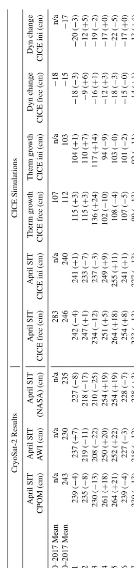
For a more robust analysis of winter ice growth during the record warm winter of 2016/2017, we now include April thickness estimates from CS2 (CPOM, AWI and NASA), the free CICE simulation and the CICE simulations initialized with CPOM CS2 November SIT in Fig. 4. Corresponding values for all other years are shown in Fig. 5 (CS2) and Fig. 6 (CICE). Table 3 summarizes associated mean April thick-ness and anomalies since 2011, together with contributions from thermodynamics (ice growth) and dynamics (ice trans-port and ridging) based on the CICE model simulations. The area for which these estimates are provided corresponds to the area shown in Fig. 1d.

Figure 4.CryoSat-2 and CICE simulated thickness anomalies in April 2017 relative to the 2011–2017 mean. The top row of panels show the total ice thickness anomalies from CryoSat-2 for CPOM(a), AWI(b)and NASA(c). Panel(d)shows April 2017 thickness anomalies from CICE initialized with CPOM November CS2 thickness together with the contributions from thermodynamics(e)and dynamics(f)and panels(h–j)shows the corresponding results from the CICE free simulations. Grid points with less than 100 individual measurements and a mean sea ice thickness of less than 0.5 m are not included.

thickness should be more accurate from CS2 than modeled estimates, robust analysis of winter ice growth from CS2 is in part limited due to the impact of climatological snow depth assumptions, which may differ from one year to the next, and differences in waveform processing between CS2 data providers, which may result in inconsistencies in the mag-nitude and direction of the observed thickness anomalies. In the free CICE simulation, November sea ice thickness is less certain, due to error accumulation during the model run. In the initialized CICE simulation, both these error sources are reduced but inherent model biases remain. While we discuss some of the regional differences below, we are most confi-dent in the model simulations on the Arctic basin-wide scale,

over which CICE has been tuned to agree with CS2 winter ice growth.

CICE-T able 3. Mean April sea ice thickness (SIT) and anomaly with respect to the 2011–2017 mean (in parentheses) from three C S2 products (CPOM, A WI and N ASA), and the CICE (free run 1985–2017) and CICE runs initialized wit h CS2 ice thickness in No v ember . The amount of thermodynamic ice gro wth and dynamical ice change from the CICE m odel runs is also gi v en. Spatial mean is o v er Arctic Basin, defined as the area sho wn in Fig. 1d. n/a – not av ailable CryoSat-2 Results CICE Simulations April SIT April SIT April SIT April SIT April SIT Therm gro wth Therm gro wth Dyn change Dyn change CPOM (cm) A WI (cm) (N ASA) (cm) CICE free (cm) CICE ini (cm) CICE free (cm) CICE ini (cm) CICE free (cm) CICE ini (cm) 1990–2017 Mean n/a n/a n/a 283 n/a 107 n/a − 18 n/a 2010–2017 Mean 243 230 235 246 240 112 103 − 15 − 17 2011 239 ( − 4) 237 ( + 7) 227 ( − 8) 242 ( − 4) 241 ( + 1) 115 ( + 3) 104 ( + 1) − 18 ( − 3) − 20 ( − 3) 2012 235 ( − 8) 219 ( − 11) 218 ( − 17) 247 ( + 1) 233 ( − 7) 115 ( + 3) 110 ( + 7) − 9 ( + 6) − 12 ( + 5) 2013 230 ( − 13) 208 ( − 22) 210 ( − 25) 234 ( − 12) 237 ( − 3) 136 ( + 24) 117 ( + 14) − 16 ( + 1) − 19 ( − 2) 2014 261 ( + 18) 250 ( + 20) 254 ( + 19) 251 ( + 5) 249 ( + 9) 102 ( − 10) 94 ( − 9) − 12 ( + 3) − 17 ( + 0) 2015 264 ( + 21) 252 ( + 22) 254 ( + 19) 264 ( + 18) 255 ( + 11) 108 ( − 4) 103 ( − 0) − 18 ( − 3) − 22 ( − 5) 2016 239 ( − 4) 227 ( − 3) 228 ( − 7) 254 ( + 8) 241 ( + 1) 107 ( − 5) 101 ( − 2) − 15 ( − 0) − 17 ( + 0) 2017 230 ( − 13) 218 ( − 12) 238 ( + 3) 233 ( − 13) 227 ( − 13) 99 ( − 13) 92 ( − 11) − 14 ( + 1) − 13 ( + 4)

ini performs better (e.g., 2012, 2014). In contrast, in 2011 and 2017 we find disagreement among the three CS2 data sets. In April 2011, both the CPOM and NASA product have overall negative thickness anomalies for the Arctic Basin (−4 and−8 cm, respectively), whereas they are positive in the AWI product (+7 cm). In April 2017, both the CPOM and AWI are in close agreement that the ice cover was overall thinner (−13 and −12 cm, respectively), as are the CICE-free and CICE-ini simulations (negative thickness anomalies of−13 cm), whereas NASA shows a weak positive anomaly (+3 cm).

Focusing more on April 2017, the three CS2 products sug-gest widespread thinner ice in April 2017 north of Ellesmere Island (up to −80 cm thinner) relative to the 2011–2017 mean (Fig. 4 top). Thinner ice is also found within the Chukchi and East Siberian seas (on average−10 to−35 cm thinner) despite a mix of positive and negative anomalies. CICE simulations, in contrast, show more widespread thin-ning throughout the western Arctic, including the Beaufort Sea and positive thickness anomalies north of Ellesmere Is-land (Fig. 4 middle and bottom). In the Beaufort Sea, there is general disagreement among the three CS2 products, as well as with the CS2 results and the CICE simulations: regional mean anomaly of −5 cm (CPOM), 0 cm (AWI), +20 cm (NASA), −25 cm (CICE-ini) and −30 cm (CICE-free). North of Ellesmere Island, CICE-ini indicates positive thickness anomalies (up to+50 cm), whereas all 3 CS2 prod-ucts show negative thickness anomalies (up to−80 cm). In this region, the CICE-free simulation also shows mostly neg-ative thickness anomalies (−20 to−80 cm), with a small pos-itive area (up to+25 cm).

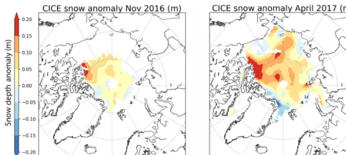
While the discrepancy in this region is puzzling, the bias between the CICE-ini simulations and the CS2 products may in part reflect the use of a snow climatology in the CS2 ness retrievals. As discussed earlier, a positive sea ice ness anomaly was found in the November 2016 CS2 thick-ness retrievals north of CAA and Greenland. Yet this positive thickness anomaly is not preserved through April in both the CPOM and AWI CS2 products. Figure 7 shows CICE sim-ulated snow depth anomalies in November 2016 and April 2017. In November, small positive snow depth anomalies oc-cur throughout the Arctic, especially north of the Queen Eliz-abeth Islands where the anomaly locally increases to 20 cm. By April, the anomalies cover a broader region and increase in magnitude. A positive April snow depth anomaly of 15 to 20 cm relative to W99 would result in an underestimation of the CS2-retrieved April ice thickness (SIT) by 88 to 115 cm using the following equation:

SIT=ρsnowHsnow+ρwaterFc

(ρwater−ρice)

,

Figure 7.Snow depth anomaly for November 2016 (relative to 2010–2016) and April 2017 (relative to 2011–2017) from CICE.

1999), ice density (ρice)of 915 kg m−3and water density of

(ρwater) 1024 kg m−3. CICE-ini, which relies on the CPOM

CS2 November thickness, maintains this positive thickness anomaly through April despite reduced thermodynamic ice growth. The CICE-free simulation, in contrast, started with negative thickness anomalies in November within this re-gion, and maintains them through April.

Conversely, thickness is also strongly influenced by dy-namics, such as convergence against the CAA and Greenland which leads to thicker ice in this region (Kwok et al., 2015). However, during winter 2017, the Beaufort High largely col-lapsed (Moore et al., 2018), reducing convergence against the northern CAA and Greenland (Fig. 8). One advantage of using CICE, is that we can more readily diagnose thermo-dynamic vs. thermo-dynamical contributions to the observed thick-ness anomalies. For the region directly north of Ellesmere Island, both the CICE-ini and CICE-free simulations sup-port reduced sea ice convergence, leading to thinner ice from dynamical contributions. At the same time, this region also exhibited reduced thermodynamic ice growth in both CICE simulations. One would expect thermodynamic ice growth to be reduced in regions of enhanced snow depth and thicker November ice. Positive snow depth anomalies extended from this region through the northern Beaufort Sea, in agree-ment with extended regions reductions in thermodynamic ice growth in both CICE-free and CICE-ini. At the same time, regions of positive 2016 November thickness anoma-lies are also associated with regions of reduced CICE ther-modynamic ice growth.

Overall, the largest reductions in thermodynamic ice growth during winter 2016/2017 occurred within the Chukchi Sea and north of the CAA, extending through the northern Beaufort Sea (in the order of−40 cm). While snow depth and thickness anomalies influenced thermodynamic ice growth north of the CCA, within the Chukchi Sea the neg-ative ice growth anomalies were a result of late ice formation: ice formed a month later than the 1981–2010 mean within the

Chukchi Sea. This seems to have been more important than increases in ice thickness from dynamics. Dynamical thick-ness changes simulated by CICE show an overall thicken-ing of the ice in winter 2016/2017 within the Chukchi and Bering seas (up to 50 cm). Anomalous ridging in this re-gion is in agreement with observed high amounts of defor-mation along the shore fast ice zone within the Chukchi Sea, as a result of persistent west winds from December to March (http://arcus.org/sipn/sea-ice-outlook/2017/june, last access: August 2017).

An exception to reduced thermodynamic ice growth oc-curs directly north of Utqia˙gvik, Alaska (formerly Barrow), with positive thermodynamic ice growth anomalies of 30 to 40 cm. This enhanced ice growth was offset by ice di-vergence, leading to overall thinner ice in the CICE sim-ulations. In situ observations of level first-year ice thick-ness off the coast of Utqia˙gvik ranged between 1.35 and 1.40 m during May (http://arcus.org/sipn/sea-ice-outlook/ 2017/june, last access: August 2017) and appear to be in better agreement with the CICE simulations, as well as the CPOM and AWI CS2 thickness estimates, while the NASA CS2 product shows positive thickness anomalies in that re-gion. Positive thermodynamic ice growth anomalies are also found for small regions north of Greenland and within Fram Strait, as well as within some scattered coastal regions of the Chukchi, East Siberian, Laptev and Kara seas.

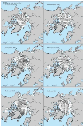
Figure 8.Mean monthly sea ice motion from the NSIDC Polar Pathfinder Data Set. Preliminary data provided by Scott Stewart, NSIDC.

to development of thin ice in newly formed open water ar-eas, increasing thermodynamic ice growth in the Laptev Sea, whereas increased ice advection from thick ice regions north of Greenland towards Fram Strait, combined with changes in internal ice stress as the ice cover has thinned, leads to more deformation. Interestingly, while the CICE model

Figure 9.Time-series from 1985 to 2017 of mean winter ice growth (mid-November to mid-April) in the free CICE simulation(a), mean 2 m NCEP-2 air temperature(b), cumulative freezing degree days (FDDs)(c)and November ice thickness(d). All time-series results are averaged over the areas shown in Fig. 1c. Corresponding images to the left of each time-series plots show the following: mean ice growth from November to April as averaged from 1985/1986 to 2016/2017; correlation coefficient between ice growth and 2 m NCEP-2 air tem-perature; correlation coefficient between ice growth and FDDs; and correlation coefficient between ice growth and November ice thickness, respectively. All correlation values are given for linear regression of de-trended time series.

Overall, for the Arctic Basin as a whole, CICE simula-tions suggest the overall thinner ice observed in April 2017 is largely result of reduced thermodynamic ice growth (−11 to−13 cm), with dynamics adding+1 to+4 cm (Table 3). 3.4 Negative feedbacks

Ice growth after the September minima is a result of turbu-lent heat flux exchanges between the relatively warm ocean

Figure 10.Standard deviation of CICE-simulated snow depth using NCEP-2 reanalysis for the month of April from 2011 to 2017.

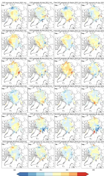
Conversely, thinner ice regions generally exhibit more vig-orous ice growth. For example, during winter 2012/2013, CICE-free, and to a lesser extent CICE-ini simulated thermo-dynamic ice growth increased throughout much of the Arctic Ocean in areas where the ice retreated in September 2012 (Fig. 6) and where the November 2012 thickness anoma-lies were negative (Fig. 3). This process of rapid winter ice growth over thin ice regions represents a negative feedback, allowing for ice to form quickly over large parts of the Arctic Ocean following summers with reduced ice cover and thinner November ice.

Thus, while summer sea ice is rapidly declining, several studies have indicated negative feedbacks over winter con-tinue to dominate (e.g., Notz and Marotzke, 2012; Stroeve and Notz, 2015), allowing for recovery following summers with anomalously low sea ice extent, such as those observed in 2007 and 2012. This is further supported in the CICE-free simulations which show the least amount of winter ice growth for the Arctic Basin in 1989, and peak ice growth following the 2007 and 2012 record minimum sea ice ex-tent (Fig. 9). As a result, mean ice growth from November to April in CICE simulations from 1985 to 2017 shows a posi-tive trend that is weakly correlated to winter air temperatures or FDDs (R=0.49). Conversely, we find a strong inverse correlation (R= −0.82) between November sea ice thick-ness and winter ice growth. Thus, because thin ice grows faster than thick ice, there is an overall stabilizing effect that suggests as long as air temperatures remain below freezing, even if they are anomalously warm, the ice can recover dur-ing winter. This stabilizdur-ing feedback over winter means that major departures of the September sea ice extent from the long-term trend caused by summer atmospheric variability

generally does not persist for more than a few years (Serreze and Stroeve, 2015).

However, since 2012, overall ice growth has declined as winter air temperatures have increased further. This not sur-prising in that there was a lot of new ice to form in the open waters left after the 2012 record minima. However, 2016 tied with 2007 for the second lowest Arctic sea ice minimum and overall thermodynamic ice growth was significantly less. The correlation from 1985 to 2012 is smaller than over the full record (R=0.34), suggesting a growing influence of warmer winter air temperatures though the difference in correlation is not statistically significant. While there remains a large amount of inter-annual variability in winter warming events, Graham et al. (2017) suggest a positive trend in not only the maximum temperature of these warming events, but also in their duration. Interestingly, there is a modest correlation be-tween detrended FDDs and the winter maxima sea ice extent (R=0.30); not removing the trend results in a correlation of R=0.83. Thus, recent reductions in overall FDDs may have played a role in the last three years of record low maxima extents.

4 Discussion

snow depth anomalies ranged from−6 to+6 cm, with a cor-responding impact of−41 to+41 cm on thickness.

Besides not accounting for inter-annual variability in snow depth, which makes assessing thickness anomalies from one year to the next less certain, differences in waveform process-ing between the three different CS2 products adds further un-certainty. The fact that the NASA CS2 product is a general outlier compared to the AWI and CPOM products is further highlighted in Fig. 11. Across the area considered (e.g., ar-eas in color shown in Fig. 1c), the difference between April and the previous November ice thickness is shown for each CryoSat-2 year. The AWI and CPOM products tend to ex-hibit positive ice growth over winter, focused north of Green-land and the CAA and sometimes also across the pole. The NASA product, in contrast, generally shows less ice growth between November and April in most years and even no ice growth in some regions. The reasons for this are unclear, yet interestingly in winter 2016/2017, all three products show more agreement in regards to thickness decreases that span a broad region north of Greenland and the CAA, combined with positive increases south of the pole towards the East Siberian and Laptev seas.

Finally, how important were the April thickness anoma-lies in the evolution of the summer ice cover in summer 2017? Several studies have discussed how thin winter ice may precondition the Arctic for less sea ice at the end of the melt season as thinner ice melts and open water ar-eas form more readily in summer, enhancing the ice albedo feedback (e.g., Stroeve et al., 2012; Perovich et al., 2008), and sea ice thickness has been used as a predictor for the September sea ice extent (Kimura et al., 2013). Thus, we may have expected 2017 to be among the lowest recorded sea ice extents as the ice cover was likely thinner than av-erage and the winter extent was the lowest in the satellite record. Nevertheless, the minimum extent ended up as the 8th lowest in the satellite data record. This highlights the continuing importance of summer weather patterns in driv-ing the September minimum. Sprdriv-ing and summer 2017 were dominated by several cold core cyclones, leading to near av-erage air temperatures and ice divergence (see http://nsidc. org/arcticseaicenews/, last access: August 2017, for a dis-cussion of this summer’s weather patterns). Overall, the cor-relation between detrended winter sea ice thickness anoma-lies and September sea ice extent remains low (Stroeve and Notz, 2015). Other factors, such as melt pond formation in spring (Schröder et al., 2014) and summer weather patterns, still largely govern the evolution of the summer ice pack at current thickness levels (e.g., Holland and Stroeve, 2011). Interestingly, predictions of the monthly mean Septem-ber 2017 sea ice extent based on spring melt pond fraction in May gave a value of 5.0±0.5 million km2, whereas the ob-served value was 4.80 million km2 (See arcus.org/sipn/sea-ice-outlook/2017/june, last access: August 2017).

5 Conclusions

In this study we examined sea ice thickness anomalies de-rived from three different CS2 data products and that were simulated using CICE. Overall freezing degree days were much reduced in winter 2016/2017, and subsequent sea ice thickness estimates from CryoSat-2 in April 2017 suggest the ice was thinner over large parts of the Arctic Ocean. These re-sults are complimented with CICE model simulations, both with and without initializing with November ice thickness distributions from CS2. While CICE simulations suggest the mean thickness within the Arctic Basin in April 2017 was the thinnest over the CryoSat-2 data record, corresponding CS2-derived sea ice thickness from the three different data providers put this into question. However, the use of CS2-derived freeboards with a snow depth climatology remains problematic because it fails to capture inter-annual snow ac-cumulation variability. Differences in processing of the radar waveform, values of snow and ice density, delineation of first-year vs. multi-year ice, and sea surface height retrieval also contribute to differences among available data sets, mak-ing it challengmak-ing to robustly assess inter-annual variability of ice thickness from CryoSat-2. Despite these challenges it is encouraging that in most years, the interannual variability in positive and negative anomalies is consistent between the three CS2 data sets.

Finally, CICE-free simulations from 1985 to 2017 reveal the correlation between winter ice growth and November ice thickness (R= −0.82) is stronger than between growth and FDDs (R=0.49), highlighting the importance of the nega-tive winter growth feedback mechanism. This supports previ-ous studies that the long-term sea ice reduction in the Arctic Basin is mainly driven by summer atmospheric conditions. However, this correlation has become weaker since 2012, in-dicating that higher winter air temperatures and further de-lays in autumn or winter freeze-up, due to warmer mixed-layer ocean temperatures, prohibit a complete recovery of winter ice thickness in spite of the negative feedback mech-anism. This is highlighted by the fact that overall thermody-namic ice growth for winter 2016/2017 was just under 1 m despite 2016 reaching the second lowest minimum extent recorded during the satellite record.

Data availability. The AWI data are available from www.

Competing interests. The authors declare that they have no conflict of interest.

Acknowledgements. This work was in part funded under NASA

grant NNX16AJ92G (Stroeve). Sea ice simulations and CryoSat-2 satellite data processing performed under NERC funding of the Centre for Polar Observation and Modeling (CPOM). CryoSat-2 thickness fields courtesy of Andy Ridout at CPOM. Processing of the AWI CryoSat-2 (PARAMETER) is funded by the German Ministry of Economics Affairs and Energy (grant: 50EE1008) and data from November 2010 to April 2017 obtained from http://www.meereisportal.de (last access: May 2017) (grant: REKLIM-2013-04).

Edited by: Chris Derksen

Reviewed by: two anonymous referees

References

Bekryaev, R. V., Polyakov, I. V., and Alexeev, V. A.: Role of polar amplification in long-term surface air temperature variations and modern Arctic warming, J. Climate, 23, 3888–3906, 2010. Bitz, C. M. and Roe, G. H.: A mechanism for the high

rate of sea ice thinning in the Arctic Ocean, J. Cli-mate, 17, 2623–2632, https://doi.org/10.1175/1520-0442(2004)017<3623:AMFTHR>2.0CO;2, 2004.

Boisvert, L. N., Petty, A. A., and Stroeve, J.: The Impact of the Extreme Winter 2015/16 Arctic Cyclone on the Barents–Kara Seas, B. Am. Meteorol. Soc., 144, 4279–4287, https://doi.org/10.1175/MWR-D-16-0234.1, 2016.

Cohen, L., Hudson, S. R., Walden, V. P., Graham, R. M., and Granskog, M. A.: Meteorological conditions in a thin-ner Arctic sea ice regime from winter through early sum-mer during the 388 Norwegian young sea ICE expedi-tion (N-ICE2015), J. Geophys. Res.-Atmos., 122, 7235–7259, https://doi.org/10.1002/2016JD026034, 2017.

Cullather, R. I., Lim, Y., Boisvert, L. N., Brucker, L., Lee, J. N., and Nowicki, S. M. J.: Analysis of the 426 warmest Arctic winter, 2015–2016, Geophys. Res. Lett., 43, 808–816, https://doi.org/10.1002/2016GL071228, 2016.

Flocco, D., Schröder, D., Feltham, D. L., and Hunke, E. C.: Impact of melt ponds on Arctic sea ice simula-tions from 1990 to 2007, J. Geophys. Res., 117, C09032, https://doi.org/10.1029/2012JC008195, 2012.

Graham, R. M., Cohen, L., Petty, A. A., Boisvert, L. N., Rinke, A., Hudson, S. R., Nicolaus, M., and Granskog, M. A.: increasing frequency and duration of Arctic win-ter warming events, Geophys. Res. Lett., 16, 6974-6983, https://doi.org/10.1002/2017GL073395, 2017.

Graversen, R. G.: Do changes in midlatitude circulation have any impact on the Arctic surface air temperature trend?, J. Climate, 19, 5422–5438, 2006.

Graversen, R. G. and Burtu, M.: Arctic amplification en-hanced by latent energy transport of atmospheric plane-tary waves, Q. J. Roy. Meteor. Soc., 142, 2046–2054, https://doi.org/10.1002/qj.2802, 2016.

Haas, C., Beckers, J., King, J., Silis, A., Stroeve, J., Wilkinson, J., Notenboom, B., Schweiger, A., and Hendricks, S.: Ice and snow thickness variability and change in the high Arctic Ocean ob-served by in situ measurements, Geophys. Res. Lett., 44, 10462– 10469, https://doi.org/10.1002/2017GL075434, 2017.

Hendricks, S., Ricker, R., and Helm, V.: User Guide – AWI CryoSat-2 Sea Ice Thickness Data Product (v1.2), hdI:10013/epic.48201. 2016.

Holland, M. M. and Stroeve, J. C.: Changing seasonal sea ice pre-dictor relationships in a changing Arctic climate, Geophys. Res. Lett., 38, L18501, https://doi.org/10.1029/2011GL049303, 2011. Hunke, E. C., Lipscomb, W. H., Turner, A. K., Jeffery, N., and El-liott, S.: CICE: the Los Alamos Sea Ice Model Documentation and Software User’s Manual Version 5.1, 2015.

Jakobshavn, E., Vihma, T., Palo, T., Jakobson, L., Keernik, H., and Jaagus, J.: validation of atmospheric reanalysis over the central Arctic Ocean, Geophys. Res. Lett., 39, L10802, https://doi.org/10.1029/2012GL051591, 2012.

Kanamitsu, M., Ebisuzaki, W., Woollen, J., Yang, S.-K., Hnilo, J. J., Fiorino, M., and Potter, G. L.: NCEP-DOE AMIP-II Reanalysis (R-2), B. Am. Meteorol. Soc., 83, 1631–1644, https://doi.org/10.1175/BAMS-83-11-1631, 2002, updated 2017. Kimura, N., Nishimura, A., Tanaka, Y., and Yamaguchi, H.: Influence of winter sea-ice motion on sum-mer ice cover in the Arctic, Polar Res., 32, 20193, https://doi.org/10.3402/polar.v32i0.20193, 2013.

Kurtz, N. and Harbeck, J.: CryoSat-2 Level 4 Sea Ice Elevation, Freeboard, and Thickness, Version 1, Boulder, Colorado USA. NASA National Snow and Ice Data Center Distributed Active Archive Center, 2017.

Kurtz, N. T., Galin, N., and Studinger, M.: An improved CryoSat-2 sea ice freeboard retrieval algorithm through the use of waveform fitting, The Cryosphere, 8, 1217–1237, https://doi.org/10.5194/tc-8-1217-2014, 2014.

Kwok, R.: Sea ice convergence along the Arctic coasts of Green-land and the Canadian Arctic Archipelago: Variability and extremes (1992–2014), Geophys. Res. Lett., 42, 7598–7605, https://doi.org/10.1002/2015GL065462, 2015.

Laxon, S. W., Giles, K. A., Ridout, A. L., Wingham, D. J., Willatt, R., Cullen, R., Kwok, R., Schweiger, A., Zhang, J., Haas, C., Hendricks, S., Krishfield, R., Kurtz, N., Far-rell, S., and Davidson, M.: CryoSat-2 estimates of Arctic sea ice thickness and volume, Geophys. Res. Lett., 40, 732–737, https://doi.org/10.1002/grl.50193, 2013.

Markus, T., Stroeve, J. C., and Miller, J.: Recent changes in Arctic sea ice melt onset, freeze-up, and melt season length, J. Geophys. Res., 114, C12024, https://doi.org/10.1029/2009JC005436, 2009.

Merkouriadi, I., Cheng, B., Graham, R. M., Rosel, A., and Granskog, M. A.: Critical role of snow on sea ice growth in the Atlantic sector of the Arctic Ocean, Geophys. Res. Lett., 44, 10479–10485, https://doi.org/10.1002/2017GL075494. 2017. Moore, G. W. K., Schweiger, A., Zhang, J., and Steele, M.:

Collapse of the 2017 winter Beaufort High: A response to thinning sea ice?, Geophys. Res. Lett., 45, 2860–2869, https://doi.org/10.1002/2017GL076446, 2018.

Overland, J. E. and Wang, M.: Recent extreme arctic tempera-tures are due to a split polar vortex, J. Climate, 29, 5609–5616, https://doi.org/10.1175/JCLI-D-16-0320.1, 2016.

Perovich, D. K., Richter-Menge, J. A., Jones, K. F., and Light, B.: Sunlight, water and ice: Extreme Arctic sea ice melt dur-ing the summer of 2007, Geophys. Res. Lett., 35, L11501, https://doi.org/10.1029/2008GL034007, 2008.

Pithan, F. and Mauritsen, T.: Arctic amplification dominated by temperature feedbacks in contemporary climate models, Nat. Geosci., 7, 181–184, https://doi.org/10.1038/ngeo2017, 2014. Polyakov, I. V., Beszczynska, A., Carmack, E. C., Dmitrenko, I. A.,

Fahrbach, E., Frolov, I. E., Gerdes, R., Hansen, E., Holfort, J., Ivanov, V. V., Johnson, M. A., Karcher, M., Kauker, F., Mori-son, J., Orvik, K. A., Schauer, U., Simmons, H. L., Skagseth, A., Sokolov, V. T., Steele, M., Timokhov, L. A., Walsh, D., and Walsh, J. E.: One more step towards a warmer Arctic, Geophys. Res. Lett., 32, L17605, https://doi.org/10.1029/2005GL023740, 2005.

Rae, J. G. L., Hewitt, H. T., Keen, A. B., Ridley, J. K., Ed-wards, J. M., and Harris, C. M.: A sensitivity study of the sea ice simulation in HadGEM3, Ocean Model., 74, 60–76, https://doi.org/10.1016/j.ocemod.2013.12.003, 2014.

Ricker, R., Hendricks, S., Helm, V., Skourup, H., and Davidson, M.: Sensitivity of CryoSat-2 Arctic sea-ice freeboard and thick-ness on radar-waveform interpretation, The Cryosphere, 8, 1607– 1622, https://doi.org/10.5194/tc-8-1607-2014, 2014.

Ricker, R., Hendricks, S., Girard-Ardhuin, F., Kaleschke, L., Lique, C., Tian-Kunze, X., Nicolaus, M., and Krumpen, T.: Satellite observed drop of Arctic sea ice growth in winter 2015–2015, Geophys. Res. Lett., 44, 3236–3245, https://doi.org/10.1002/2016GL072244, 2017a.

Ricker, R., Hendricks, S., Kaleschke, L., Tian-Kunze, X., King, J., and Haas, C.: A weekly Arctic sea-ice thickness data record from merged CryoSat-2 and SMOS satellite data, The Cryosphere, 11, 1607–1623, https://doi.org/10.5194/tc-11-1607-2017, 2017b. Rigor, I. G., Wallace, J. M., and Colony, R. L.:

Re-sponse of sea ice to the Arctic Oscillation, J. Cli-mate, 15, 2648–2663, https://doi.org/10.1175/1520-0442(2002)015<2648:ROSITT>2.0.CO;2, 2002.

Schröder, D., Feltham, D. L., Flocco, D., and Tsamados, M.: September Arctic sea-ice minimum predicted by spring melt-pond fraction, Nat. Clim. Change, 4, 353–357, https://doi.org/10.1038/NCLIMATE2203, 2014.

Screen, J. A. and Simmonds, I.: The central role of diminishing sea ice in recent Arctic temperature amplification, Nature, 464, 1334–1337, 2010.

Serreze, M. C., Barrett, A. P., Stroeve, J. C., Kindig, D. N., and Holland, M. M.: The emergence of surface-based Arctic ampli-fication, The Cryosphere, 3, 11–19, https://doi.org/10.5194/tc-3-11-2009, 2009.

Stroeve, J. and Notz, D.: Insights on past and future sea-ice evo-lution from combining observations and models, Global Planet. Change, https://doi.org/10.1016/j.gloplacha.2015.10.011, 2015. Stroeve, J. C., Serreze, M. C., Kay, J. E., Holland, M. M., Meier,

W. N., and Barrett, A. P.: The Arctic’s rapidly shrinking sea ice cover: A research synthesis, Climatic Change, 135, 119–132, https://doi.org/10.1007/s10584-011-0101-1, 2012.

Stroeve, J. C., Markus, T., Boisvert, L., Miller, J., and Bar-rett, A.: Changes in Arctic Melt Season and Implica-tions for Sea Ice Loss, Geophys. Res. Lett., 110, 1005, https://doi.org/10.1002/2013GL058951, 2014.

Tilling, R. L., Ridout, A., Shepherd, A., and Wingham, D. J.: In-creased arctic sea 454 ice volume after anomalously low melting in 2013, Nat. Geosci., 8, 643–646, 2015.

Tilling, R. L., Ridout, A., and Shepherd, A.: Near-real-time Arctic sea ice thickness and volume from CryoSat-2, The Cryosphere, 10, 2003–2012, https://doi.org/10.5194/tc-10-2003-2016, 2016. Tilling, R. L., Ridout, A., and Shepherd, A.: Estimating Arctic

sea ice thickness and volume using CryoSat-2 radar altimeter data, Adv. Space Res., https://doi.org/10.1016/j.asr.2017.10.051, 2017.

Tsamados, M., Feltham, D. L., Schröder, D., Flocco, D., Farrell, S., Kurtz, N., Laxon, S., and Bacon, S.: Impact of variable atmo-spheric and oceanic form drag on simulations of Arctic sea ice, J. Phys. Oceanogr., 44, 1329–1353, https://doi.org/10.1175/JPO-D-13-0215.1, 2014.

Tsamados, M., Feltham, D., Petty, A., Schröder, D., and Flocco, D.: Processes controlling surface, bottom and lateral melt of Arctic sea ice in a state of the art sea ice model, Philos. T. R. Soc. A, 373, 2052, https://doi.org/10.1098/rsta.2014.0167, 2015. Warren, S. G., Rigor, I. G., Untersteiner, N., Radionov, V. F.,

Bryaz-gin, N. N., Aleksandrov, Y. I., and Barry, R.: Snow depth on Arc-tic sea ice, J. Climate, 12, 1814–1829, 1999.