SRef-ID: 1607-7946/npg/2004-11-281
Nonlinear Processes
in Geophysics
© European Geosciences Union 2004
Null modes effect in Rossby wave model
V. Goncharov1and V. Pavlov2
1Institute of Atmospheric Physics, Russian Academy of Sciences, 109017 Moscow, Russia
2UFR de Math´ematiques Pures et Appliqu´ees, Universit´e de Lille 1, 59655 Villeneuve d’Ascq, France Received: 8 July 2003 – Revised: 1 April 2004 – Accepted: 5 April 2004 – Published: 28 May 2004
Abstract. The problem of the null-modes existence and some particularities of their interaction with nonlinear vortex-wave-like structures is discussed. We show that the null-modes are fundamental elements of nonlinear wave fields. The conditions under which null-modes can mani-fest themselves are elucidated. The Rossby-Hasegawa-Mima (RHM) model is used for the illustration of features of null-modes-waves interactions.
1 Introduction
The purpose of the paper is to consider features of wave in-teractions in inhomogeneous, anisotropic, nonlinear media in a case when proper values,ωk,for interacting wave modes, ak,turn to zero in some domain ofk-space. We present a
new approach to solving the problem based on the Hamil-tonian formulation of fluid dynamics (see Appendix A). We analytically study a new class of structures that can exist in two-dimensional flows governed by equations similar to the Rossby-Hasegava-Mima (RHM) ones (Hasegava and Mima, 1977; Kadomtsev, 1965; Similon and Sudan, 1990; Krall and Trivelpiece, 1973; Petviashvili and Pohotelov, 1989). These structures, termed below null-modes, turn out to be an im-portant element in the theory of wave interactions and pro-voke a variety of intriguing questions. One task is to un-derstand what physical reality corresponds to the basic state (null-modes) of the wave system when the proper values,ωk,
for interacting wave modes,ak,become zero in some domain
of thek-space. Another one is to explore how the presence of null-modes modifies the wave interaction process as com-pared to the analogous well-studied process in homogeneous media. Finally, how does one develop field variables for the proper functions evolving in such a situation? Answers to these questions are of fundamental interest because so far all
Correspondence to: V. Pavlov
modern theories of wave interactions have been formulated in terms of normal modesak.
Before proceeding further, let us remind the reader that the concept of interacting waves is extensively used in wave physics and provides explanations for numerous collective effects. Its essence is that wave interaction is effectively real-ized only when the so-called resonance conditions on phases (frequencies and wave vectors) of interacting waves are sat-isfied (see for example Zakharov et al., 1985 and references therein).
For instance, in hydrodynamical systems, as experiments show (see Kadomtsev, 1965; Petviashvili and Pohotelov, 1989, and References therein), stationary flows sometimes appear as a result of intense field fluctuations. In geophysics, it is well-known that stationary (zonal) flows in atmospheres of rotating planets always coexist with intense surrounding wave fields. Based on the analogies from other branches of wave physics, it was once natural to assume that one of the principal mechanisms for stationary flow generation is the nonlinear interactions of waves. However, in geophys-ical hydrodynamics, application of the traditional approach to concrete situations is sometimes accompanied by difficul-ties. For example, the attempt to explain the appearance of stationary flows in the framework of three-wave resonance interaction of waves governed by the Rossby equations has failed: it has been shown that such a three-wave mechanism of interactions cannot be responsible for generation of sta-tionary flows (see Longuet-Higgins and Gill, 1969; Pedlosky, 1986).
This theoretical result has instigated the approach which is developed below.
The canonical version of the HA uses the following ba-sic assumptions: the system under consideration is described by a set of canonical variables, symbolically marked here bypandq.Generally, more than one pair of variables ex-ists. The Fourier transformation of field variables from x-space into k-space, (p, q)→(pk∗, qk) is achieved, in
or-der to identify the spectral wave components. A disper-sion relationship between the frequency and the wave vec-tor of the components is given byω=ωk.Normal variables, ak, ak∗,are introduced by a linear transformation from(p, q)
to(ak, ak∗)as coefficients for developing p, q over
corre-sponding eigenfunctions,fk(x).In a homogeneous medium,
fk(x)∼expik·x.The Hamiltonian of the system is the full energy expressed in terms of canonical variables,H[p, q].
In terms of normal variables, the quadratic part of the Hamiltonian developed in a functional series with respect to field variables, H[p, q]=H2+H3+... , is presented as
H2=Rdkωkaka−kand equations for normal modes
evolu-tion have the form∂tak=−iδH /δak∗and∂tak∗=+iδH /δak.
Here, ak∗=a−k, δH /δu is a functional derivative with
re-spect to field variableu.One assumes that 0<H[p, q]<+∞,
which means that there are not of field perturbations at infin-ity: a physical problem of wave interactions is always con-sidered in terms of wave packets.
Difficulties do not arise when the frequency of a wave mode depends on the absolute value of the wave vec-tor, ωk=ω|k|, i.e. when the medium is homogeneous and isotropic. In this case, the HamiltonianH2 is positive and remains positive when transformationk→−kis made. Diffi-culties appear when the media is anisotropic and proper value
ωk depends on any particular direction, for example, when ωk∼kx. Such a dependence follows, for instance, from the
linearized version of Eq. (6). Obviously, in this case, result-ing frequency cannot be simply introduced into the expres-sion forH2becauseH2becomes null in this case. There is also no support or a motivated physical reason for including the absolute value|ωk|intoH2.
For this reason only, a detailed analysis of the problem is essential.
The paper aims to achieve several goals: (i) to formulate, in a brief and relatively complete form, the fundamentals of one of the Hamilton approach versions; (ii) to formulate the concept of normal modes when the Hamiltonian of a system is defined by an operator expression; (iii) to introduce the canonical variables; (iv) to apply the developed methodology to the enigmatic physical phenomenon. It should be noted that without complying with certain rules, the procedure for introducing canonical variables, and normal variables as a consequence, is not as elementary as it could be expected.
In this article we perform the study in terms of general-ized potentials (“canonical” field variables)p andq, when the transition from field variables (velocities components)
(v1, v2) to (p, q) is carried out, on the one hand, with-out a decrease of phase space dimension and, on the other hand, complying with the gauge invariance of the theory (see Sect. 3).
The article is structured as follows: Sect. 2 specifies the basic model and establishes some general results. In Sect. 3, we discuss the canonical formulation of the Hamiltonian de-scription for fluid dynamics of nonlinear, dispersive, non-homogeneous media. The Hamiltonian formulation for a Rossby-Hasegawa-Mima-like wave model is also proposed. The crucial importance of the proper introduction of normal variables in such systems is highlighted in Sect. 4. We con-sider the RHM-model as an example to which the HA can be directly applied to obtain analytical results. In Sect. 5, we discuss a linear approximation and explain where the null-modes hide. In Sect. 6, the features of three-wave inter-actions are analyzed. A nonlinear collision of three wave packets is considered in Sect. 7. The null-mode mechanism of flow generation is considered in Sect. 8 and in Sect. 9, where all obtained results are discussed. In summary, we have found that specific structures (null-modes) can exist in strongly nonlinear and anisotropic wave systems. These not evolving in time structures (in linear approximation with re-spect to fields perturbations) correspond to the basic phys-ical state when the stream-function, 9,is zero. The struc-tures cannot be uncovered when one works with linearized equations, and, in some sense, they may be considered as “sleeping” ones. However, their presence can be observed when nonlinear interactions are taken into account with spe-cific resonant conditions. One goal of the work was to find the conditions when such structures could be brought to light, in order to experimentally observe a generation of null-modes (i.e. observe the phenomenon of generation of time-independent flows by interacting wave fields). The real-ization of these conditions is so difficult that without prelim-inary theoretical analysis the effect may neither be guessed, nor observed experimentally.
2 Basic model
We consider a two-dimensional fluid motion, typical exam-ples of which are large scale horizontal motions in planet atmospheres, hydrodynamical motions of a strongly magne-tized plasma, etc. Such motions are described in the frame-work of the two-dimensional model of an incompressible perfect fluid. The velocity field is characterized in such a sit-uation by two components only,v=(v1, v2,0). The suppres-sion of the third velocity component,v3,can be caused by several physical causes. The evolution equations in this case are traditionally formulated in terms of generalized vortic-itywhich is introduced by the relation=curlv.For two-dimensional motions, only one component of vorticity,3,is not null. The condition of incompressibility,divv≡∂ivi=0,
permits to introduce the stream-function,9,via the relation
vi=ij∂j9,wherei, j=1,2, ij is an antisymmetrical unit
tensor,12=1= −21, 11=22=0.
The evolution of two-dimensional vorticity-like systems are governed by the equation
which can be written as
∂t= −(∂2ψ )∂1+(∂1ψ )∂2, (2) The right part of this equation can be rewritten in terms of Jacobian, J[a, b], where the Jacobian is defined as
J[a, b]=∂1a ∂2b−∂2a ∂1b≡ij∂ia∂jb. Equation (2)
con-serves the full energy of the fluid motion
H= 1 2
Z
dxρψ . (3)
We suppose that all field variables and their derivatives, i.e. all perturbations, vanish in infinity. Also, background sta-tionary flows are presumed to be absent.
The generalized vorticity,, and the stream-function,ψ,
are related in general case by the operator relationship
= ˆL9. (4)
The specification of a concrete physical model is assured by a relation between the stream-function and vorticity.
So, for a two-dimensional Euler equation, the indicated relationship has the form=−1ψ,i.e.Lψˆ ≡−1ψ.Here,
1=∂x2+∂y2the two-dimensional Laplacian. Below we will frequently usex≡x1, y≡x2.
There exist other models (for example, the mod-els of so-called “screened” vortices) with the operator
ˆ
L=−(1−1/a2),whereais some space scale defined by the choice of the model. Such models are largely used to de-scribe (i) different plasma motions based on the Hasegawa-Mima equation ((Hasegava and Hasegawa-Mima, 1977; Similon and Sudan, 1990)), (ii) axial electronic vortices (Krall and Triv-elpiece, 1973), (iii) the quasi-geostrophic barotropic motions (see below), etc. There exist even more complex examples (Gruzinov, 1992).
Let us provide as an illustration one visual example. In the geo-astrophysical context, it is typical to use a quasi-geostrophic barotropic model defined by the relationship
= ˆL9+βy, β =2ω0
a cosϑ0. (5)
Here,Lˆ can be given byLˆ=−(1−1/a2). The term linear iny accounts, in the first approximation, for the sphericity effect (β-effect), i.e. the variation of the Coriolis force with latitudeϑ.Equation (5) is used in analyzing large-scale mo-tions in an atmosphere considered as a thin layer of a fluid rotating with the angular velocityω0. Let us note that Eq. (2) describes in this context two-dimensional fluid motions even ifLˆ and9depend on the vertical coordinatez.
Equations (2–4) form the closed system of equations for
, 9.
Below, we consider the simplest case of two-dimensional motions where the stationary density,ρs=ρ0,is independent on the vertical coordinatez.In the integralH,after integrat-ing onz, z-dependence vanishes. Choosing mass, distance, time scales for whichρ0=1, a=1, β=1 and scaling the full
energy to obtain a dimensionless expression forH,the di-mensionless stream-function,ψ, will be governed by the di-mensionless evolution equation in the planex, y
∂t(1−1)ψ+∂xψ+J[ψ, 1ψ] =0. (6)
where the vorticity and the stream-function are related by the relationship
= −(1−1)ψ+y. (7)
The full energy of the fluid is then transformed into
H →H =1 2
Z
dxψ = −1 2
Z
dxψ (1−1)ψ. (8)
3 Hamiltonian approach
The model governed by Eqs. (2–4) (see also Eqs. (6–8)) illus-trates the Hamiltonian system with a finite number of fields and with a continual number of degrees of freedom charac-terized by the indexx.For this reason, functional derivatives with respect to field variables are used. To address the is-sue we use the version of the HA given in Goncharov and Pavlov (1984, 1993, 1997, 1998, 2001, 2002) and Pavlov et al. (2001). Information on supplementary bibliography can be found in Zakharov et al. (1985).
We will call the system a Hamiltonian one if it evolves according to
∂tui = {ui, H} =
Z
dx0{ui, u0j}
δH
δuj(x0)
. (9)
Here, the Hamiltonian of the system, H, is the quantity-energy-functionally dependent on the fields,ui,the operator
δ/δuis the operator of the functional derivative. The deriva-tives of dynamical variables, F[u], are calculated by using the relationδui(x)/δuj(x0)=δijδ(x−x0).
The Hamiltonian structure of the system described by Eq. (9) includes the Hamiltonian given by the total energy,
H, and the functional Poisson bracket {. , .}. This bracket is antisymmetric, bilinear, and satisfies the functional Jacobi identity presented symbolically in the following form {A, {B , C}} + {B,{C , A}} + {C,{A , B}} =0, (10) Condition Eq. (10) must be obligatory satisfied for Hamilto-nian systems.
Conservation of energy follows from the given formula-tion of governing equaformula-tions, since−∂tH={H, H}=0.
3.1 Noncanonical formulation
Systems which evolve according to Eqs. (2–4), give an ex-ample of such Hamiltonian systems. In fact, Eqs. (2–4) can be rewritten as
∂t= {, H} =
Z
dx0{, 0}δH
Let us show how the bracket{, 0}is calculated for con-crete situations. Using expressions (8) and (11), we obtain that
{, H} = Z
dx0ψ0
, 0 . (12)
Here and further, the prime indicates that a field variable depends on the primed two-dimensional space coordinate x0=(x0, y0).On the other hand, using Eq. (2), we can exclude
∂tfrom Eq. (11). The following step is to introduce the
Ja-cobian under the integration operator where the properties of delta function are used. The regrouping of the integrand terms (all field variables vanish at infinity) yields
Z
dx0ψ0J δ x−x0
, −, 0 =0. (13) The expression in the square brackets is zero because Eq. (13) is satisfied for anyψ.Therefore, the Poisson bracket for the potential vorticitycan be written as
, 0 =J δ x−x0 ,
. (14)
This expression satisfies the Jacobi requirement, Eq. (10), which are necessary for Poisson brackets. The result, Eq. (14), can be obtained also by the direct calculation of the bracket on the canonical basis.
However, the formulation in terms of vorticity is some-times uncomfortable because the Poisson bracket for such systems is functionally dependent of the field variables. By this reason, the canonical formulation of the problem is sometimes more preferable.
3.2 Canonical formulation of RHM-like wave model The initial physical system is described by evolution equa-tions of Euler which are formulated in terms of “measurable” physical variables, i.e. in terms of velocitiesv1, v2. Below, we will describe the same system in terms of canonical vari-ablesp, qfor which the functional Poisson brackets have the form :
p, q0 =δ(x −x0),
p, p0 =q, q0 =0,i.e. when the corresponding Poisson’s brackets for field variables are independent on field variables. Such a choice is presented as more “natural” because the transitionv1, v2→p, qconserves the same number of field variables, i.e. the same dimension of the phase space. In this case, an evolution of the system based on Eq. (6) will be described by an alternative, cano-nical, form. It signifies that the canonical variables satisfy equations
∂tq=
δH
δp, ∂tp= − δH
δq, (15)
where the HamiltonianH, the total energy expressed in terms of canonical field variablesp, q,is given by
H= −1 2 Z
dxψ (p, q)(1−1)ψ (p, q), (16) and whereψ is expressed in terms ofq, p. Variablesq, p
have the meaning of the generalized coordinate and momen-tum, respectively.
In this context, some comments on the subject must be made.
What is the essence of the proposal “to introduce canoni-cal variables”? Obviously, one possible way is to express the field variables, for examplevi,in terms of generalized
poten-tials,p, q,which satisfy some (canonical) conditions. Thus, the problem is reduced to a search of a functional dependence
vi[p, q].The dependence and corresponding canonical
vari-ables of such a type are known as Clebsh representations. It was A. Clebsh (1859) who pioneered using of similar trans-formations for a hydrodynamical velocity in an incompress-ible fluid (see for example Lamb, 1932). For some (sim-plest) systems, the canonical variables (potentials)q andp
for incompressible fluid are introduced by vk=∂k8+p∂kq
(a review of more complex situations is given in Goncharov and Pavlov (1993)). Constraint divv=0 signifies that the potential 8 can be eliminated from consideration because for an incompressible fluid we have18=−∂i(p∂iq). The
vorticity is defined via the Clebsh potential by the expres-sioni=εij k∂jp∂kq.For two-dimensional flows, i=3 and
the tensor Levy-Civitaεij k becomes ε3j k≡εj k.However, it
is clear that there is some functional arbitrary rule for choos-ing of a canonical basis (p, q)for the given physical field
vi.To remove this arbitrary rule, one postulates that the
the-ory must possess the gauge invariance. The criterion for removing the arbitrary rule is a possibility of the existence of such canonical transformations under which all physical (measured) quantities of the theory are kept invariant. This principle is called the principle of gauge invariance, gener-ates in turn some specific laws of conservation which elim-inate an over-determination of the system. The existence of such laws means, from a geometrical standpoint, that an evo-lution of the system is realized on some surface in the sym-plectic spacep, qwhich is fixed by indicated lows of conser-vation.
One can show that the relationship between the velocity components v1, v2 and the potentialsp, q is given by the sufficiently cumbersome nonlinear differential-integral ex-pression
(1−1) vk =εkn∂n εij∂iq∂jp+∂2p+x2∂1q, (17) Let us demonstrate this formula for a single pair of cano-nical variablesp,q,i.e. for plane flows when only one pair of potentials is used. In this case, we have:
=J (p, q)=εij∂ip∂jq. (18)
The variablesq,pcomposing the canonical basis have mean-ing of the canonical coordinate and the canonical momen-tum, respectively. Thus, evolution equations formulated in terms of canonical variablesp,q are given by
∂tp= −
δH
δq , ∂tq = δH
δp. (19)
After calculating the functional derivatives ofH,one finds that
Let us consider a quasi-geostrophic model (see Sect. II) withβ6=0 The basic dimensionless relationship between the stream-function and the generalized vorticity is given by
= ˆLψ+x2, (21)
which is expressed by Eq. (18) too. For this reason, we have the expression which gives a relationship between the stream-function and canonical variablespandq
ˆ
Lψ+x2=J (q, p) . (22)
Let us suppose now that a state of dynamical equilibrium ex-ists. The equilibrium values of variables corresponding to this state are marked by indexs.Let us suppose that the back-ground flow is absent, i.e.ψs=0. However, even ifψs=0,
the problem arises for determining the nontrivial equilibrium values for the canonical variables (see for example Gon-charov, 1984). So, we can find from Eqs. (20) and (18) that the stationary state,ψs=0,is determined by
∂tps =0, ∂tqs =0, (23)
x2=J (ps, qs) , (24)
where Eq. (24) follows from the two definitions of the vor-ticity presented above. Evidently, the solutions of Eq. (23) are two time-independent functions which satisfy only one Eq. (24). For this reason, we can choose one of the potentials
ps orqs arbitrarily. Choosing the functionpsas
ps =x1, (25)
we obtain
qs =
1 2x
2
2. (26)
All physical (“measurables”) fields do not change in this case.
Now, it is convenient to introduce new canonical variables
p0=p−ps, q0=q−qs, (27)
which in the equilibrium regime satisfy to the condition
p0s=qs0=0.
In terms of perturbationsp0,q0,relationship (18) and (20) are written as
ˆ
Lψ=x2∂1q0+∂2p0+J q0, p0
, (28)
∂tq0=
δH δp0 =J q
0+
x1, ψ, (29)
∂tp0= −
δH δq0 =J
1 2x
2 2+p
0
, ψ
. (30)
Omitting the prime, one sees that Eq. (28) is transformed into Eq. (17) if we apply to Eq. (28) operatorεij∂j.
Let us move now into k-space, using the symmetric Fourier transforms defined by the formula
Zk= Z dx
2πZ(x)exp(−ik·x).
The goal of such a transformation is, first, to obtain the dis-persion relationship for wave components and, second, to ap-ply the results of the theory to interacting wave components with fixed wave vectors.
In this case, according to Eqs. (15–17), the Fourier com-ponents evolution is governed by nonlinear equations
∂tqk= δH δp∗k, ∂tp
∗
k = −
δH
δqk, (31)
The asterisk(∗)denotes the complex conjugate.
Concerning a possibility of the Fourier transformations, we have supposed that the background flows are absent and all field variables (perturbations) vanish rapidly in infin-ity, i.e. even|x|ψ→0 when|x|→∞.Such a supposition is largely used in the framework of traditional approaches in physics when models of wave packets are considered. In this case, all physical operators are transformed according toA(ˆ x,∇)→ ˆAk(−i∇k, ik).Multiplying Eq. (17) by the
ex-ponent, integrating over the space coordinate and neglecting terms in infinity, we can find that the stream-function com-ponentψk and the canonical variables’ componentsqk,pk
are related by the relationship
ψk = − 1 k2+1
iσpk−κ∂qk ∂σ
+ Z dk
1dk2
2π qk1pk2(σ1κ2−σ2κ1)δ(k1+k2−k)
. (32) Here,κ andσ are longitudinal and transversal components of the wave vectork, i.e.k=(κ, σ ).The operators act on all variables which are positioned to the right of them.
The Hamiltonian is given by the simple expression
H[p, q] = 1 2
Z
dkk2+1|ψk|2, (33) where the function ψk has to be expressed in terms of the canonical variablesqk,pk.
The Hamiltonian Eq. (33) is the functional polynˆomial of the fourth order with respect to field (canonical) variablesqk,
pk.It can be written as
H[p, q] =H2[p, q] +H3[p, q] +H4[p, q], (34) whereH2[p, q]describe linear effects, andH3,4[p, q] non-linear effects of interacting perturbations into the system.
4 Normal variables
The problem of introducing normal variables is not trivial because operator combinations appear in Eq. (32). Similar combinations will appear inH2[p, q].
Let us write Eqs. (31) in a matrix form
∂tuk= −iJˆ δH
where +
denotes the Hermitian conjugate. The column vectorsuk and so-called symplectic matrix Jˆare arranged
as u=
pk qk
, Jˆ=
0−i i 0
. (36)
The Poisson brackets can be written as n
uk,u+
k0
o
= −iJ δˆ k−k0
. (37)
Let us consider small field perturbations relative to basic unperturbed state. In this case, the leading term into the HamiltonianH is the quadratic termH2[p, q]with respect to canonical variablesp andq.This approximation corre-sponds to the linear approximation for evolution equations. ForH2[p, q],we can write the following representation
H2= 1 2 Z
dk u+kHˆkuk, (38)
The matrix operatorHkˆ have the following structure ˆ
Hk =
Ak Bkˆ ˆ Bk+Ckˆ
, (39)
where matrix elementAk is a function of σ andκ, while elementsBkˆ andCkˆ are operators. These elements are ex-pressed by
Ak= σ
2
k2+1, (40)
ˆ Bk=
iσ κ
k2+1
∂ ∂σ,
ˆ Ck = −
∂ ∂σ
κ2
k2+1
∂
∂σ. (41)
By definition (see below), normal variablesak(t )are in-troduced as coefficients in decomposition
uk= ˆfkak+ ˆf
∗ −ka
∗
−k, (42)
wherefk,f∗−kare vector-column eigenfunctions.
In terms of normal variables, the two equations of evolu-tion Eq. (35) are transformed into
∂tak= −i
δH δa∗k, ∂ta
∗
k=i δH δak
. (43)
In linear approximation,H→H2. The Hermitian matrix operator Hˆk at Eq. (38) has a typical structure Eq. (39).
Considering the fact that Hˆ is Hermitian, H2 is real, and uk=u∗−k,one sees that
ˆ
Hk = ˆHk+= ˆH
∗ −k.
It means that ˆ
Ak= ˆA+k = ˆA∗−k, Ckˆ = ˆCk+= ˆC−∗k, Bkˆ = ˆB−∗k. (44) Substituting Eq. (38) into the Hamiltonian Eqs. (35), we obtain the linear equation
ˆ
J ∂t+iHkˆ
uk=0. (45)
To formulate the problem on eigenfunctions and eigenval-ues, we must substituteuk= ˆfkexp(−iω t )in Eq. (45),
as-suming that, in general, the eigenvectors fˆk are operators non-commuting with the eigenvaluesω=ωk. In doing so, we obtain
ˆ
Hkfˆk− ˆJfˆkωk =0, (46)
It should be noted that as far asfˆkωk6=ωkfˆk,this prob-lem cannot be reformulated in the form
ˆ
Hk−ωkJˆfˆk=0
which is traditional for expressions with no operators. Using the propertiesHˆk= ˆH−∗k, Jˆ=− ˆJ
∗, we can derive from Eq. (46) the dual linear problem
ˆ
Hkfˆ∗−k+ ˆJfˆ∗−kω−k=0. (47)
Comparing Eq. (46) with Eq. (47) shows that ifωkandfˆk are an eigenvalue and an eigenvector then−ω−k andfˆ
∗ −k
are too. Therefore, all the eigenvalues and the eigenvectors of problem Eq. (46) have dual nature and can be split into such pairs. In the simplest case when a model has only one wave branch, the problem Eq. ( 46) has a single pair of eigen-vectorsfˆk,fˆ∗−kand a corresponding pair of eigenvalues
(ωk,−ω−k).
In this case, according to general theory tenets (Goncharov and Pavlov, 1993), because matricesHkˆ andJˆare Hermitian and, in addition,Hkˆ is positively determined, there are good grounds for believing that, on the one hand, the eigenvec-torsfˆk andfˆ∗−k form the system of orthonormal functions
subjected to the conditions ˆ
f+kJˆfˆ
k=1, fˆ
+
kJˆfˆ
∗
−k =0, (48)
on the other hand, all the eigenvalues are real, i.e.=ωk=0. Thus, normal variablesak(t )are introduced as coefficients in decomposition of the column vectorukon the
eigenvec-torsfˆk,fˆ∗−kby Eq. (42).
Using orthonormality property Eq. (48), from Eq. (42) it is easy to obtain the relations
ak = ˆf+kJˆu
k= −u+−kJˆfˆ
∗
k, (49)
and next, by employing Eq. (37), to calculate {ak, ak∗0} = −iδ k−k0
, {ak, ak0} =0. (50)
On the basis Eq. (50), the matrix equation of motion Eq. (35) takes form
∂tak= −i
δH δa∗k, ∂ta
∗
k=i δH δak
. (51)
To find solutions forfˆ andωkin an explicit form in what
follows we assume for simplicity that matrix elementAkis
In this case one can show that according to Eq. (46) eigen-vectorfˆkis given by
ˆ
fk= −A −1
k
ˆ Bk+iωk
1
!
εk, (52)
The eigenvalueωkand the normalizing factorεk, in turn,
can be found from orthonormality conditions Eq. (48) which is convenient to reformulate, using Eq. (52), as
ωk−ω−k= −i
AkBˆk+A−1k − ˆBk, (53)
ω−kωk =Ak
ˆ
Ck− ˆBk+A−1k Bkˆ
, (54)
|εk|2=(ωk+ω−k)−1Ak. (55)
Here,ωkis the eigenvalue of the problem,εkis a normaliza-tion coefficient. To find the eigenvalueωkand the normaliz-ing factorεk,we must resolve conditions Eqs. (53–55) with Eqs. (39) and (41), which lead to
ωk−ω−k= − κ
k2+1, (56)
ω−kωk =0, (57)
|εk|2= σ
2
k2+1(ωk+ω−k)
. (58)
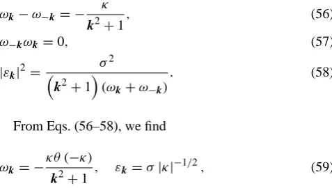
From Eqs. (56–58), we find
ωk= −κθ (−κ) k2+1 , εk
=σ|κ|−1/2, (59)
whereθ (κ)is the Heaviside function:θ (κ)=1 ifκ≥0,and
θ (κ)=0 ifκ<0. This law of wave dispersion is shown in Fig. 1. For κ≤0 it describes the well-known Rossby-like waves. The domain ofκ>0 corresponds to so-called null modes.
Summing up this section, we list the basic relationships
qk =σ|κ|−1/2 ak−a−∗k
, (60)
pk= −i|κ|1/2sign (κ)
∂
∂σ + θ (κ)
σ
ak
− ∂
∂σ + θ (−κ)
σ
a∗−k
. (61)
The stream-function is defined via the normal variables by expression
ψk = − |κ|−1/2 ωkak+ω−ka−∗k
− 1
2πk2+1 ×
Z
dk1dk2pk2qk1(σ1κ2−σ2κ1) δ (k−k1−k2) . (62)
wherepk, qkhave to be expressed by Eq. (61).
-8
4
8 -4
0
κ
σ
Fig. 1. A general dispersion law for the Rossby-like waves and null
modes.
5 Linear approximation
In the linear approximation, when interaction of Rossby-like waves is ignored, the Hamiltonian takes form
H2= Z
dkωk|ak|2>0, (63)
and, as earlier discussed, is positively defined sinceωk≥0 in accordance with Eq. (59). Due to the presence ofθ (−κ) -function in the dispersion law Eq. (59), null modes defined above as normal modes with positive components ofκ, are eliminated in a linear approximation. Once initially estab-lished, these modes remain unchanged without any phys-ical consequences or effects because, in accordance with Eq. (62), in a linear approximation we have
ψ (x)= − 1 2π Re
Z
dk|κ|−1/2ωkakeikx
≡ψR+ψN M, (64)
and hence they make zero contribution to the stream-function,ψN M=0,even if their amplitudes are distinct from zero.
As we shall see later, this is no longer the case in a nonlin-ear approximation.
The null-modes correspond to the state with9=0. How-ever, using the traditional consideration where governing equations are formulated in terms of a stream-function, it is very difficult to guess to which physical reality the states with9=0 correspond. On the other hand, discovering that the stream-function 9=9[p, q] depends in reality on ca-nonical field variables (p, q) which arise from transition
6 Three-wave interactions
To find the types of wave interactions admissible by normal waves dispersion Eq. (59), we must consider resonance con-ditions which take null modes into account. Becauseωk≥0, and hence the so-called waves of the negative energy are ab-sent, the main contribution at the first order of perturbation theory is made by the three-wave interactions corresponding to the resonance conditions
k−k1−k2=0, ωk−ωk1−ωk2 =0, (65) which describe decay processes (0→1+2) and inverse processes-merging(1+2→0).
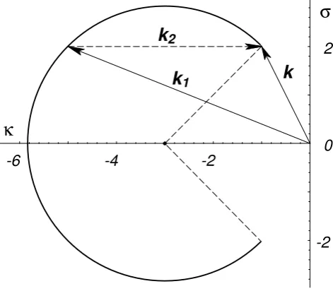
Of special interest are the interactions between two Rossby-like waves and a null mode which arise whenever one of wave-vectors, for examplek2, has a positive compo-nentκ2while componentsκandκ1are negative. In this case, wave-vectors of interacting Rossby-like modes form a locus where
ωk=ωk1. (66)
According to Eq. (66), the tips of vectorskandk1must lie on the circle with radiusr=
q
ωk−2/4−1 and the center at point
−ωk−1/2,0as graphically represented in Fig. 2.
In order to proceed further, we must also know the Hamil-tonian of the three-wave interactions which is responsible for resonance Eq. (65), and ignore all other feasible non-resonant terms which can be eliminated with the aid of the canonical transformation. Thus, we arrive at the Hamiltonian with a general structure
H3= 1 2 Z
dkdk1dk2 ak∗ak1ak2Vk,k1,k2)+c.c
×δ (k−k1−k2) , (67) where functionVk,k1,k2is called the interaction factor or cou-pling coefficient. The coucou-pling coefficientVk,k1,k2 can be obtained by expanding Eq. (33) into a functional power se-ries of normal variables with subsequent collecting of terms proportionate toa∗aa and aa∗a∗. Because our interest is only in resonance interactions, functionVk,k1,k2 is defined only on the surface described by Eq. (65). Therefore, if we restrict ourselves to the three-wave interactions, terms pro-portional to(ωk−ωk1−ωk2)can be omitted in the computa-tion ofVk,k1,k2.
After some algebra, we find
Vk,k1,k2 =
i (σ1κ2−κ1σ2) 2π√|κκ1κ2|
ωk1σ2−ωk2σ1
× κ
σθ (κ)+ κ1
σ1
θ (κ1)+
κ2
σ2
θ (κ2)
+ ωk1κ2−ωk2κ1
−(σ1κ2−κ1σ2)
× ∂ω
k ∂σ −
∂ωk1 ∂σ1
−∂ωk2 ∂σ2
. (68)
-6
-4
-2
σ
-2
0
2
κ
k
1k
2k
Fig. 2. Locus of the null-mode wave-vector tails merging with a
Rossby-like mode. Dashed-line vectork2denotes the null mode,
solid-line vectorskandk1denote the Rossby-like modes.
7 Nonlinear collision of three wave packets
We consider the interaction of three narrow-band wave pack-ets whose typical wave-vectorsk1,k2, k3 satisfy the reso-nance conditions
k1=k2+k3, ωk1 =ωk2 +ωk3. (69) Let us assume that
a (k)=a1(k)+a2(k)+a3(k) ,
where each ofanis nonzero only ifq=k−knare small. Fast
dependence ontandxfor each wave packet is excluded with transformation
cn(q)=an(kn+q)expi ωknt−knx
.
Following the standard procedure (see, e.g. Zakharov and Kuznetsov, 1986), using new variables
un(x)=(2π )−1
Z
dqcn(q) eiq·x
which have significance of complex envelopes for wave-trains, and using a band narrowness of the wave packets, we obtain
H = i 2
3 X
n=1 vn
Z
dxun∇u∗n+V
Z
dxu∗1u2u3+c.c., (70) where envelope velocities vn and interaction coefficient V
which is a function of the wave-vectorsk1,k2,k3, are ex-pressed as
vn=∂ωkn/∂kn
=k2n+1 −2n
κn2−σn2−1,2κnσn
o
, (71)
Now, let us consider interaction between two Rossby-like wave packetsk,k1and the null mode packetk2. So far as in this caseκ1, κ2<0 butκ3>0, from Eq. (68) we have
V = −i (σ2κ3−κ2σ3) 2
2π√|κ1κ2κ3| ∂ω
k1 ∂σ1
−∂ωk2 ∂σ2
. (73)
The space-time evolution of the packets can be described from equations
∂tuj = −i
δH δu∗j,
which take the form
∂tu1+v1∇u1= −iV u2u3,
∂tu2+v2∇u2= −iV∗u1u∗3,
∂tu3= −iV∗u∗2u1. (74)
8 Null-mode mechanism of flow generation
As shown by Longuet-Higgins and Gill (1969), the mech-anism of a direct triad resonance which takes into account only Rossby-like modes, cannot be responsible for exciting zonal flows if weak corrections for sideband resonance are ignored. This conclusion is completely confirmed by our re-sults and is readily apparent from Eq. (68) whereby coupling coefficientVk1,k2,k3 vanishes ask1=k2.
As will be shown later, in contrast to the cited works, our approach which uses the null-mode concept admits the gen-eration of zonal flows due to direct triad resonance Eq. (69) involving two Rossby-like wave packetsk1,k2and a packet of null modek3.These resonances are governed by the sys-tem of three nonlinear Eqs. (69) which in general can be solved by inverse scattering method when initial envelopes are non-overlapping. Using this technique, Zakharov (1976) obtained special solution describing a physically important effect – a parametric decay of a pump wave into secondary waves.
8.1 Noncoplanar casev1×v26=0
Consideru1,u2as envelopes of Rossby-like waves fixed in the initial stage at t→−∞ when the null-mode packet u3 is absent. Then, using characteristic coordinates τ1, τ2,τ3 defined as
x= −v1τ1−v2τ2, t = −τ1−τ2−τ3, (75) Zakharov’s solution can be presented in the form
u1= 1
V
f2f3 1+(F1+F2) F3
,
u2= 1
V
f1f3 1+(F1+F2) F3
,
u3= −
i V
f1∗f2F3 1+(F1+F2) F3
, (76)
where fi=fi(τi) are arbitrary, square-integrable, complex
functions, andFiare determined by
F1= +∞ Z
τ1
ds |f1|2, F2=
τ2 Z
−∞
ds |f2|2,
F3= +∞ Z
τ3
ds |f3|2. (77)
To interpret correctly the initial-value problem in terms of characteristic coordinatesτ1,τ2,τ3, we note that due to the minus signs in Eq. (75), fixing any two of the characteristic coordinates would send the third characteristic coordinate to +∞ift→−∞, or to−∞ift→+∞. Thus, the initial states will be located where any one of the characteristic coordi-nates approaches+∞, and the final states will be located where any one of the characteristic coordinates approaches +∞. Therefore, quantities
u+i = lim
τi→+∞
ui, u−i =τ lim
i→−∞
ui, (78)
correspond to the initial and final profiles, respectively. Considering the integral characteristic
Ii+= Z
dxu+i 2
, Ii−= Z
dxu−i 2
(79) as initial and final intensities of the packets, we can obtain a convenient formula for their calculation
Ii±=si
g1/2 V
× Z
dτjdτk∂j∂kln 1+(F1+F2) F3|τi=±∞
, (80)
wheresi=sign ∂iFi andg1/2=
q
v21v22−(v1v2)2is the Jaco-bian of transformation Eq. (75).
Denoting
Yi =
Z +∞
−∞
ds |fi|2, i=1,2,3, (81)
we can compute the initial and final integral intensities of the wave packets.
As shown by Zakharov (1976), in the initial stage when the wave packetu3is absent, the integral intensities ofu1,
u2, andu3are determined as
I1+= −g 1/2
V Z
dτ2dτ3∂2∂3ln(1+F2F3)
=g 1/2
V ln(1+Y2Y3) , (82)
I2+=g 1/2
V Z
dτ2dτ3∂1∂3ln(1+(F1+Y2) F3)
=g 1/2
V ln
1+ Y1Y3 1+Y2Y3
, (83)
In final stage we have all three packets with intensities
I1−= −g 1/2
V Z
dτ2dτ3∂2∂3ln(1+(Y1+F2) F3)
=g 1/2
V ln
1+ Y2Y3 1+Y1Y3
, (85)
I2−=g 1/2
V Z
dτ2dτ3∂1∂3ln(1+F1F3)
=g 1/2
V ln(1+Y1Y3) , (86)
I3−= −g 1/2
V Z
dτ2dτ3∂1∂2ln(1+(F1+F2) Y3)
=g 1/2
V ln 1+
Y32Y1Y2
1+Y3(Y1+Y2) !
. (87)
It is convenient to introduce the renormalized intensities
Ji±=g−1/2V Ii± (88)
Then, eliminating quantitiesY1,Y2, Y3from Eqs. (82–87), we can express final intensitiesJi− (i=1,2,3)in terms of the initial ones as
J1−=J1++J2+−lnh1+eJ1+
eJ2+−1i, (89)
J2−=lnh1+eJ
+
1
eJ
+
2 −1i, (90)
J3−= −J2++lnh1+eJ1+
eJ2+−1i. (91)
8.2 Coplanar case
In a coplanar case whenv1×v2=0,Eqs. (74) become ˙
u1+v1∂u1/∂ξ = −iV u2u3, (92) ˙
u2+v2∂u2/∂ξ = −iV∗u1u∗3, (93) ˙
u3= −iV∗u1u∗2. (94)
and describe the evolution in time and one spatial dimension of the three-wave resonant interaction. The spatial variable
ξ used as a coordinate along the line of propagation v1, is related toxby expression
ξ =xcosϕ+ysinϕ, (95)
As shown in Fig. 2, angleϕdefines the direction of the prop-agation(−π/2<ϕ<π/2). Together with frequencyω1, it can be used for parameterization of the resonant triplet
k3=2r (cosϕ,sinϕ) , (96) k1,2= −
1 2ω1
(1,0)±1
2k3, (97)
wherer= q
ω−21 /4−1.
We consider the situation when in the initial stage at
t→−∞, Rossby-like wave packetsu1,u2are localized at in-finities(ξ=±∞)and the null-mode packetu3is absent. Ve-locities of the wave packets can be evaluated from relations
v1,2= |∂ωk/∂k|k=k1,2 =
4ω31r
2ω1rcosϕ∓1
. (98)
which show thatv1<0 andv2>0. Thus, these packets move towards each other and after some time collide generating null-mode packet u3. At the final stage at t→∞, when Rossby-like wave packets run away into infinities, all that re-mains in the interaction region is the immovable null-mode packetu3 which will never leave the place of its creation. This situation corresponds to the special solution
u1= − 2p1
√
−v1(v2−v1)
V D
×
eη2 +p1v1−p2v2 p1v1+p2v2
e−η2
, (99)
u2= − 2p2
√
v2(v2−v1)
V D
×
eη1 −p1v1−p2v2 p1v1+p2v2
e−η1
, (100)
u3= −i
4p1p2(v2−v1) √
−v1v2
V (p1v1+p2v2) D
, (101)
where
η1=p1(ξ−v1t−ξ1) , (102)
η2=p2(ξ−v2t−ξ2) , (103)
D= eη1 +e−η1
eη2+e−η2
− 4p1p2v2v1 (p1v1+p2v2)2
e−η1−η2, (104)
Solutions of this sort were first considered by Zakharov and Manakov (1973). According to Eqs. (99) and (100), wave packetsu1,u2are characterized by arbitrary amplitudesb2, but the widths of the packets are related. From Eqs. (102) and (103) it follows that iflis the width of packetu1,the width of packetu2isv1/v2times smaller, where in accordance with Eq. (98),v1/v2≥1.
9 Estimates and conclusion
After the two original wave packets,u1andu2, beat against each other for some time, they escape from the interaction region leaving behind the null-mode packet,u3. Thus, at the final stage, in accordance with Eq. (76), we have the residual field
¯
a=u−3 = −i V
f1∗f2Y3
1+(F1+F2) Y3
. (105)
Because this disturbance is immovable, it will never leave the place of its creation.
Using Eq. (76) and assuming thata¯ is a slow variable, i.e.
∂a/∂x¯ =∂a/∂y¯ =0, we can compute residual fields. At first, from Eqs. (60) and (61), we obtain
q =σ3|κ3|−1/2a¯exp(ik3x)+c.c., (106)
p= −κ3|κ3|−1/2
y+ i σ3
¯
Next, from Eq. (17) we find the stream-function
ψ= ¯ψexp(2ik3x)+c.c., (108) where its envelopeψ¯ is expressed as
¯
ψ=iσ3|κ3| ¯a 2
4k23+1 . (109)
To gain greater insight into the physical significance of the results, we make some numerical estimates for an ocean model. In geostrophic approximation, the basic parame-ters are defined as a=√gh/f, β=∂2f, where f, g and
h denote the Coriolis force, the acceleration of gravity and the mean depth of layer. Choosing a=50 km (baro-clinic Rossby radius), we consider middle latitudes where
β=10−13cm−1s−1. Then, in accordance with Eq. (5), we find the scales of lengthLand time T under which model parametersaanβbecome unity:
L=a=50 km, T =(βa)−1=2·106s. (110) Let us suppose that in the initial state two Rossby-wave packets with wave vectors k1={−1.59,2.45} and k2={−5.45,1.41} move with velocities v1={−0.049,−0.086} and v2={0.025,−0.014}, and have ψ10=1.2·10−2 and ψ20=2.6·10−5, respectively. As numerical simulation shows, these packets generate a null-mode packet withk3={3.86,1.03}andψ30=2.3·10−4.
Let us conclude with a few remarks. In this paper, we have considered the simplest model which possesses both strong dispersion and strong inhomogeneity and nonlinear-ity. However, this model has permitted us to show how the null-mode concept changes traditional ideas about the influ-ence of nonlinear interactions. We have also discussed the basis for the proposed approach and highlighted important non-trivial generalization for the operator expressions of nor-mal variables.
The choice of the method is motivated by several reasons. Successful solution of a problem of theoretical physics often depends on which descriptive formalism, i.e. the mathemati-cal framework, is chosen (see Zakharov, 1985). In fact, there may exist several analytical approaches which under consis-tent application lead to the same final result. Theoreticians, however, often tend to be biased in favor of one while instinc-tively resisting attempts aiming to explore others: they claim that new approaches do not contribute anything new. Con-sequently, not all possible analytical frameworks are treated equally and some get pushed out by the others. As an exam-ple, in medieval times European universities developed sev-eral coexisted algorithms for arithmetic division, but all of them except for the single one are obsolete nowadays. How-ever, the prevailing method should not be the one that is most habitual. The “best” scheme should be the one that is most adequate for the problem in question. In fact, after the pe-riod of implementation and adaptation, the framework itself may start affecting the style of thinking and enriching sci-entific language. Finally, it may begin to define the way in which new physical problems are stated. This happened, for
instance, with the Feynmann diagram technique which orig-inally seemed to be merely a simplification method in the perturbation theory.
The analogous situation has happened with the HA which is based on the fundamental fact that governing equations of a hydrodynamical system possess a hidden Hamiltonian structure.
Appendix A Hamilton approach
There exist different methods which use the adjective ”Hamiltonian”, and there are numerous papers with titles where the adjective “Hamiltonian” is used. That is why, when talking about the Hamiltonian method, it is neces-sary to define more precisely which one of the versions is implied. The so-called “Hamiltonian principle” and the so-called “Hamiltonian description” can mean different ap-proaches.
The point of the departure for one of the approaches is the integral (action) of a hydrodynamical system taken in the form
S= Z
dtL[ui, ∂tui]
≡ Z
dt{ Z
dxAˆj[u; x,x1]∂tuj(x1)
−H[u]}. (A1) Here,Lis the Lagrangian of the hydrodynamical system,H
is the Hamiltonian of the same system, ∂tuk is the partial
derivative of a field variable with respect to time. Variations of the action,S,with respect to hydrodynamical field vari-ablesu=(uk)lead to the evolution equationδS=0,which is
equivalent to Z
dx1ωˆik[u;x,x1]∂tuk(x1)=
δH δui(x)
. (A2)
Here, δ/δum are the operator of functional derivation,
ωik is the symplectic form defined by the condition
ˆ
ωik[x,x1]=δAˆi[u(x1)]/δuk(x)−δAˆk[u(x)]/δui(x1). The approach proceeding from the extremum of Eq. (A1) and based on the use of equations Eq. (A2) has a wide dis-semination. Reviews on applications of the variational prin-ciple of least action with a hydrodynamical Lagrangian den-sity, can be found in works of Bretherton (1970); Henyey (1983); Salmon (1988) (see also publications relevant to this aspect in Abarbanel et al. (1986); Holm et al. (1985) and ref-erences therein; in context of the Hamiltonian formulation of Rossby wave model see for instance Lynch (2002)).
The other version of the Hamiltonian description proceeds from the evolution equations in the form
∂tui(x)= {ui, H}
≡ Z
dx1{ui(x), uj(x1)}
δH δuj(x1)
. (A3)
seems to be preferable sometimes from the physical point of view since it arises naturally in many known hydrodynamical models.
A particular case, the canonical form of the Hamilton ap-proach, is given by the set of equations in terms of functional derivatives
∂tqi =
δH δpi
, ∂tpi = −
δH δqi
, (A4)
whereqi, pi, i=1,2, ...N are canonical variables, andH is
the Hamiltonian of the system.
Equations (A2) and (A3) would become equivalent if there existed a one-to-one transformation, i.e. if there existed rela-tion
Z
dx2ωˆij[u;x1,x2] {uj(x2), uk(x3)}
=δikδ(x1−x3). (A5)
Such a scenario is realized when the functional Poisson brackets are non-degenerated. In this case, it would be ab-solutely irrelevant which of the formulations was taken as a point of departure.
However, for systems with degenerated functional Poisson brackets{uj, u0k}, which admit solutions of{uj, Ck}=0 for
CasimirsCk, transformations Eq. (A5) are impossible. Such
a situation is observed for hydrodynamical models (see, for example, Arnold, 1978).
If from the beginning one is forced to work within the class of models determined by evolution Eqs. (A2), it is necessary to go through the process not only of searching for the ca-nonical variables, but also ascertaining their connection with physically-observed field quantities (for example, one needs to elucidate the sense of multi-valued Clebsch representa-tions), then invent models of hydrodynamic systems with un-usual properties, and so on.
Even if the necessary structure of the Lagrangian is guessed or selected in some intuitive way, the use of the vari-ational principle Eq. (A1) requires the formulation of addi-tional postulates concerning latent constraints, the physical interpretation of which is not always obvious.
In the historical context, the Hamiltonian description in the forme of Eq. (A3) is directly driven from physically-based presumptions about the type of evolution of hydrodynami-cal systems and their internal properties (see Goncharov and Pavlov, 1997).
The Hamiltonian approach Eq. (A3) was initially devel-oped in fluid dynamics mainly for pragmatic goals, as a me-thod of solving some concrete hydrodynamical problems. For example, it appears to be very effective in finding non-linear evolution equations for interacting waves (for details, see Zakharov et al., 1985). It was immediately noticed that the Hamiltonian method possesses a number of advantages in comparison with traditional approaches. In particular, a) the Hamiltonian approach is not tied to a particular choice of “field coordinates”. Specific features of a medium turn out to be unessential to a large extent; b) many versions of the per-turbation theory may be simplified and standardized; c) the
method is rather economical because an asymptotic expan-sion can be made in the beginning; d) the physical meaning of the results of calculations obtained for a particular system can be easily revealed. In early 1970s, (see work Zakharov and Faddeev, 1971), it became apparent that the majority of nonlinear evolution equations integrated by the inverse scat-tering method possess a Hamiltonian structure, i.e. they are the infinite-dimensional analogues of the Hamilton equations of classical mechanics.
Approximately at the same time the general physical es-sence of the Hamiltonian approach was realized. It became clear that in classical physics many of the conservative mod-els which use a field concept, possess a hidden Hamilto-nian structure. Many hydrodynamical models happened to be among them.
The construction and successful use of canonical vari-ables for studying surface gravity waves Zakharov (1968) presented one of the most impressive examples of the ap-plication of the Hamiltonian approach in hydrodynamics and gave an impetus to elaborate the general wave theory for non-linear, dispersive media in the framework of the canonical Hamiltonian formalism. The issue of determining canonical variables was essential to the development of the Hamilto-nian method. For many fluid dynamic systems, the canonical variables in Clebsch representation have been introduced in an intuitive way (examples are given in Seliger and Whitham, 1968; Zakharov and Kuznezov, 1997). There even exists an opinion that the canonical variables may only be guessed (see L’vov, 1994). In reality, it is not correct, there exists a regu-lar procedure for finding canonical variables (see Goncharov and Pavlov, 1993, 1997).
If the Hamiltonian approach Eq. (A3) merely offered a new vision of familiar results, it would deserve little atten-tion. However, enough evidence has accumulated that the Hamiltonian approach, together with the methods of mod-ern classical mechanics (see Dubrovin and Novikov, 1989; Arnold, 1978), comprise a powerful tool for fluid dynamics research. Conservation laws, stability conditions, asymptotic approximations and useful variable transformations, all ac-quire logical motivation and transparency that is often lack-ing when the correspondlack-ing manipulations are applied di-rectly to the traditional evolution equations.
Acknowledgements. This work was partly supported by the
Rus-sian Foundation for Basic Research (grant No.00–05–64019–a). The authors thank A. Dyment and E. P. Tito for useful remarks.
Edited by: A. R. Osborne Reviewed by: two referees
References
Abarbanel, H. D. I., Holm, D. D., Marsden, J. E., and Ratiu, T. S.: Nonlinear stability analyzis of stratified fluid equilibria, Phyl. Trans. Roy. Soc., London A 318, 349–409, 1986.
Bogoljubov, N. N. and Shirkov, D. B.: Introduction to the Theory of Quantized Fields, 3rd Ed., Interscience, 1959; Wiley, 1980. Bretherton, F. P.: A note on Hamilton’s principle for perfect fluids,
J. Fluid Mech., 44(1), 19–31, 1970.
Dirac, P. A. M.: Generalized Hamiltonian dynamics, Proc. Roy. Soc., A 246, 326–332, 1958.
Dubrovin, B. A. and Novikov, S. P.: Hydrodynamics of weekly de-formed soliton latices: Differential geometry and Hamiltonian theory, Russ. Math. Surveys., 44 (6), 35–124, 1989.
Goncharov, V. P.: Hamiltonian representation of the equations of hydrodynamics and its use for describing wave motions in shear flows, Izvestiya Acad. Sci. USSR, Atmos. Ocean Phys., 20 (2), 92–99, 1984.
Goncharov, V. P. and Pavlov, V. I.: Problems of hydrodynamics in Hamiltonian description, Moscow University Press, Moscow, 1993.
Goncharov, V. P. and Pavlov, V. I.: Some remarks on the physical fondation of the Hamiltonian description of fluid motions, Eur. J. Mech. B/Fluids, 16 4, 509–555, 1997.
Goncharov, V. P. and Pavlov, V. I.: On the Hamiltonian approach: Applications to geophysical flows, Nonl. Proc. in Geoph., 1, 219–240, 1998.
Goncharov, V. P. and Pavlov, V. I.: Large-scale vortex structures in shear flows, Eur. J. Mech. B/Fluids, 19, 831–854, 2000. Goncharov, V. P. and Pavlov, V. I.: Multipetal vortex structures
in two-dimensional models of geophysical fluid dynamics and plasma, Journ. Exper. and Theor. Physics, 119 (4), 685–699, 2001.
Goncharov, V. P., Gryanik, V. M. and Pavlov, V. I.: Venusian “hot spot”: physical phenomenon and its quantifiation, Phys. Rev., E 66, 066304–1–066303–11, 2002.
Gruzinov, A. V.: Contour dynamics of the Hasegawa-Mima equa-tion, JETP Lett., 55, 1, 75–78, 1992.
Hasegawa, A. and Mima, K.: Stationary spectrum of strong turbu-lence in magnetized nonuniform plasma, Phys. Rev. Lett., 39, 205–208, 1977.
Henyey, F. S.: Hamiltonian description of stratified fluid dynamics, Phys. Fluid, 26 (1), 40–47, 1983.
Holm, D. D., Marshden, J. E., Ratiu, T., and Weinstein, A.: Non-linear stability of fluid and plasma equilibria, Phys. Rep., 123, 1–116, 1985.
Kadomtsev, B. B.: Plasma turbulence, Academic, New York, 1965. Krall, N. A. and Trivelpiece, A. W.: Principles of Plasma Physics,
McGrew-Hill Book Company, 1973.
Lamb, H.: Hydrodynamics, Cambridge University Press, Cam-bridge, 1932.
Longuet-Higgins, M. S. and Gill, A. E.: Proc. Roy. Soc., A 299, 120, 1969.
Lundgreen, T. S.: Hamilton’s variational principle for perfectly con-ducting plasma continuum, Phys. Fluid, 6 (7), 898–904, 1963.
L’vov, V. S.: Wave Turbulence Under Parametric Excitation,
Springer Series in Nonlinear Dynamics, Springer-Verlag Berlin Heidelberg, 1994.
Lynch, P.: Hamiltonian methods for geophysical fluid dynamics: An introduction, IMA, Univ. of Minnesota, Preprints 1838, 1– 32, 2002.
Pavlov, V. I., Buisine, D., and Goncharov, V. P.: Formation of vortex clusters on a sphere, Nonl. Proc. in Geoph., 8, 9–19, 2001. Pedlosky, J.: Geophysical fluid dynamics, 2nd Ed., Springer-Verlag,
New York, 1986.
Petviashvili, V. I. and Pohotelov, O. A.: Solitary waves in plasma and atmosphere, Energoatomizdat, Moscow, 1989.
Salmon, R.: Hamiltonian fluid mechanics, Ann. Rev. Fluid Mech., 20, 225–256, 1988.
Seliger, R. L. and Whitham, G. B.: Variational principles in contin-uum mechanics, Proc. R. Soc. London, A 305, 1–25, 1968. Similon, P. L. and Sudan, R. N.: Plasma turbulence, Annu. Rev.
Fluid Mech., 22, 317, 1990.
Zakharov, V. E.: Stability of periodic waves of finite amplitude of the surface of a deep fluid, J. Appl. Mech. Tech. Phys., 2, 190– 194, 1968.
Zakharov, V. E.: Exact solutions to the problem of the parametric interaction of three-dimensional wave packets, Sov. Phys. Dokl., 21, 322, 1976.
Zakharov, V. E. and Faddeev, L. D.: The Korteweg-de Vries equa-tion as Hamiltonian system, Func. An. and Its Appl., 5, 4, 18–27, 1971.
Zakharov, V. E. and Kuznetsov, E. A.: Hamilton formalizm for sys-tems of the hydrodynamic type, edited by Novikov, S. P., Sov. Sci. Rev., 91, 1310, 1986.
Zakharov, V. and Kuznezov, E.: Hamiltonian formalism for nonlin-ear waves, Physics-Uspekhi, 40 (11), 1137–1167, 1997. Zakharov, V. E. and Manakov, S. V.: On resonant interaction of
wave packets in non-linear media, JETP Lett., 18, 243–247, 1973.