University of Pennsylvania
ScholarlyCommons
Publicly Accessible Penn Dissertations
2018
Linear/non-Linear Types For Embedded
Domain-Specific Languages
Jennifer Paykin
University of Pennsylvania, [email protected]
Follow this and additional works at:
https://repository.upenn.edu/edissertations
Part of the
Computer Sciences Commons
This paper is posted at ScholarlyCommons.https://repository.upenn.edu/edissertations/2752
Recommended Citation
Paykin, Jennifer, "Linear/non-Linear Types For Embedded Domain-Specific Languages" (2018).Publicly Accessible Penn Dissertations. 2752.
Linear/non-Linear Types For Embedded Domain-Specific Languages
Abstract
Domain-specific languages are often embedded inside of general-purpose host languages so that the
embedded language can take advantage of host-language data structures, libraries, and tools. However, when the domain-specific language uses linear types, existing techniques for embedded languages fall short. Linear type systems, which have applications in a wide variety of programming domains including mutable state, I/ O, concurrency, and quantum computing, can manipulate embedded non-linear data via the linear type !σ. However, prior work has not been able to produce linear embedded languages that have full and easy access to host-language data, libraries, and tools.
This dissertation proposes a new perspective on linear, embedded, domain-specific languages derived from the linear/non-linear (LNL) interpretation of linear logic. The LNL model consists of two distinct fragments---one with linear types and another with non-linear types---and provides a simple categorical interface between the two. This dissertation identifies the linear fragment with the linear embedded language and the non-linear fragment with the general-purpose host language.
The effectiveness of this framework is illustrated via a number of examples, implemented in a variety of host languages. In Haskell, linear domain-specific languages using mutable state and concurrency can take advantage of the monad that arises from the LNL model. In Coq, the QWIRE quantum circuit language uses linearity to enforce the no-cloning axiom of quantum mechanics. In homotopy type theory, quantum transformations can be encoded as higher inductive types to simplify the presentation of a quantum equational theory. These examples serve as case studies that prove linear/non-linear type theory is a natural and expressive interface in which to embed linear domain-specific languages.
Degree Type
Dissertation
Degree Name
Doctor of Philosophy (PhD)
Graduate Group
Computer and Information Science
First Advisor
Steve Zdancewic
Keywords
Domain-specific language, Linearity, Quantum computing, Type system
Subject Categories
LINEAR/NON-LINEAR TYPES
FOR EMBEDDED DOMAIN-SPECIFIC LANGUAGES
Jennifer Paykin
A DISSERTATION
in
Computer and Information Science
Presented to the Faculties of the University of Pennsylvania
in
Partial Fulfillment of the Requirements for the
Degree of Doctor of Philosophy
2018
Supervisor of Dissertation
Steve Zdancewic
Professor of Computer and Information Science
Graduate Group Chairperson
Lyle Ungar
Professor of Computer and Information Science
Dissertation Committee
Stephanie Weirich, Professor of Computer and Information Science, University of Pennsylvania Benjamin Pierce, Professor of Computer and Information Science, University of Pennsylvania Andre Scedrov,Professor of Mathematics, University of Pennsylvania
LINEAR/NON-LINEAR TYPES
FOR EMBEDDED DOMAIN-SPECIFIC LANGUAGES
COPYRIGHT
2018
Jennifer Paykin
This work is licensed under a Creative Commons Attribution 4.0 International License. To view a copy of this license, visit
Acknowledgment
I have so many people to thank for helping me along the journey of this PhD. I could not
have done it without the love and support of my partner and best friend, Jake, who was
there for me every single step of the way. I also need to thank my parents Laurie and Lanny
for giving me so many opportunities in my life, and my siblings Susan and Adam for helping
me grow.
I owe so much thanks to advisor Steve Zdancewic, who has been an amazing advisor
and who has made me into the researcher I am today. Steve, thank you for teaching me
new things, encouraging me to succeed, listening to my ideas, and waiting patiently until I
realized you were right all along.
I have been lucky to have many excellent mentors over the years. Thank you to Norman
Danner, for introducing me to programming languages and pushing me to take advantage
of the opportunities that come my way. Thank you to Stephanie Weirich, for inspiring me
and supporting me over the years. Thank you to Benjamin Pierce, for making me into a
better writer, speaker, and researcher. Thank you to the rest of my thesis committee—Peter
Selinger and Andre Scedrov—for your feedback and encouragement. Finally, thank you to
Neel Krishnaswami, Dan Licata, Val Tannen, and all my other collaborators, professors,
and mentors for teaching me so much over the years.
My time at Penn would have been much less enjoyable without the wonderful friends I
have made here. To everyone at PLClub, Monday night quizzo, cisters, and GETUP, thank
you for your friendship, your commiseration, and your support. So many people have made
my life better at Penn that I cannot possibly list them all, but I need to single out my closest
confidants and conspirators—Antal, Leo, Robert, and Kenny. Thanks for everything!
Finally, my work has been supported financially by the following sources, whose
contri-butions have been much appreciated: the NSF Graduate Research Fellowship Grant Number
ABSTRACT
LINEAR/NON-LINEAR TYPES
FOR EMBEDDED DOMAIN-SPECIFIC LANGUAGES
Jennifer Paykin
Steve Zdancewic
Domain-specific languages are often embedded inside of general-purpose host languages
so that the embedded language can take advantage of host-language data structures,
li-braries, and tools. However, when the domain-specific language useslinear types, existing
techniques for embedded languages fall short. Linear type systems, which have
applica-tions in a wide variety of programming domains including mutable state, I/O, concurrency,
and quantum computing, can manipulate embedded non-linear data via the linear type !σ.
However, prior work has not been able to produce linear embedded languages that have full
and easy access to host-language data, libraries, and tools.
This dissertation proposes a new perspective on linear, embedded, domain-specific
lan-guages derived from the linear/non-linear (LNL) interpretation of linear logic. The LNL
model consists of two distinct fragments—one with linear types and another with non-linear
types—and provides a simple categorical interface between the two. This dissertation
iden-tifies the linear fragment with the linear embedded language and the non-linear fragment
with the general-purpose host language.
The effectiveness of this framework is illustrated via a number of examples, implemented
in a variety of host languages. In Haskell, linear domain-specific languages using mutable
state and concurrency can take advantage of the monad that arises from the LNL model. In
Coq, theQwirequantum circuit language uses linearity to enforce the no-cloning axiom of
quantum mechanics. In homotopy type theory, quantum transformations can be encoded as
higher inductive types to simplify the presentation of a quantum equational theory. These
examples serve as case studies that prove linear/non-linear type theory is a natural and
TABLE OF CONTENTS
ACKNOWLEDGMENT. . . iii
ABSTRACT. . . iv
1 Introduction. . . 1
1.1 Conventions . . . 9
2 Linear type systems . . . 10
2.1 A simple linear type system . . . 11
2.2 Linear connectives . . . 13
2.3 The exponential modality ! . . . 18
2.4 Dual Intuitionistic Linear Logic . . . 21
2.5 Indexed modalities . . . 23
2.6 Kind-based linear logic . . . 27
2.7 Linear/non-linear logic . . . 30
3 Embedded linear/non-linear types. . . 36
3.1 A linear embedded language . . . 36
3.2 The linear/non-linear interface . . . 39
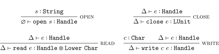
3.3 Example: linear file handles . . . 41
3.4 Monadic programming . . . 42
3.5 Extensions . . . 47
3.6 Example: session types . . . 50
3.7 Discussion . . . 54
4 Haskell Implementation . . . 56
4.2 Linear types and type checking . . . 60
4.3 Running linear programs . . . 69
4.4 Monadic programming . . . 78
4.5 Example: Arrays . . . 82
4.6 Example: Session types . . . 87
4.7 Discussion and Related Work . . . 92
5 Embedded categorical semantics . . . 98
5.1 Background . . . 98
5.2 Categories for multiplicative additive linear logic . . . 103
5.3 Linear/non-linear categories . . . 105
5.4 Embedded meta-theory . . . 106
5.5 Conclusion . . . 110
Case study: Quantum Computing 112 6 A quantum/non-quantum type system. . . 113
6.1 Quantum computing background . . . 117
6.2 The quantum/non-quantum (QNQ) calculus . . . 122
6.3 Examples . . . 126
6.4 Denotational semantics . . . 130
7 Quantum equational theories in HoTT. . . 134
7.1 Background and main ideas . . . 135
7.2 Equational theory of QNQ . . . 138
7.3 Deriving equational rules in homotopy type theory . . . 142
7.4 Equivalence of unitaries . . . 146
7.5 Denotational Semantics . . . 155
7.6 Discussion . . . 158
8 Qwire: Quantum circuits in Coq . . . 160
8.1 The Qwirecircuit language . . . 161
8.2 Linear type checking in Coq . . . 165
8.3 Surface language . . . 168
8.4 Discussion . . . 174
9 Future work . . . 177
9.1 Adapting LNL to other substructural type systems. . . 177
9.2 Formalizing the theory of embedded languages. . . 180
9.3 Variations to the structure of LNL . . . 180
9.4 Drawing on the host language . . . 180
9.5 Shortcomings and outstanding problems . . . 181
9.6 Conclusion . . . 181
LIST OF ILLUSTRATIONS
1.1 The linear/non-linear embedded programming model. . . 6
2.1 Linear implication . . . 13
2.2 Multiplicative product ⊗ . . . 14
2.3 Proof thatLUnit is the unit of ⊗. . . 15
2.4 Multiplicative unit LUnit . . . 16
2.5 Additive product . . . 16
2.6 Additive unit: LTop . . . 17
2.7 Additive sum . . . 17
2.8 Additive unit: LZero . . . 18
2.9 The linear/non-linear categorical model. The model consists of two categories related by functorsLiftandLowerthat form a categorical adjunctionLift⊣ Lower; for details see Section 5.3. . . 31
2.10 LNLLift connective . . . 32
2.11 LNLLower connective . . . 33
3.1 Specification of an embedded linear lambda calculus as terms of typeLExp∆σ. 38 3.2 Interface of linear file handles, given as inference rules, writing ∆⊢e∶σ for e∶LExp ∆σ. . . 41
3.3 Recursive types in the linear embedded language . . . 48
3.4 Polymorphism in the linear embedded language . . . 49
3.5 Dependent types in the linear embedded language . . . 50
3.6 Linear interface to session types. . . 51
4.2 Haskell interface to linear additive connectives . . . 67
4.3 Examples of linear programs embedded in Haskell . . . 68
4.4 Values in the deep embedding associated with various linear connectives. . . 74
4.5 Interface to linear arrays. . . 83
4.6 Linear quicksort algorithm . . . 88
5.1 β and η equivalence for the embedded linear lambda calculus. . . 107
6.1 Multiplicative exponential fragment of QNQ . . . 123
6.2 Quantum teleportation. . . 129
6.3 Quantum Fourier transform in QNQ . . . 130
7.1 Structural axioms . . . 141
7.2 Groupoid axioms . . . 141
7.3 Unitary equivalence axioms for X∶ U(Qubit,Qubit),SWAP∶ U(σ⊗τ, τ ⊗σ), and DISTR∶ U(σ⊗ (τ1⊕τ2),(σ⊗τ1) ⊕ (σ⊗τ2)). . . 142
7.4 Operations on open linear types . . . 148
7.5 Inductive presentation of open type equivalence. . . 150
7.6 Proofs of EquationsSWAP-introand SWAP-elim. . . 154
8.1 Unitary and non-unitary gates inQwire. Different gate sets could have been chosen, for example by picking a different universal set of unitary gates, or by allowing arbitrary circuits to be frozen as gates, which is a feature allowed by many practical circuit languages. Rennela and Staton (2018) propose some extensions to Qwire that expand the gate set to add sums and recursive data types. . . 162
8.2 Translation of QNQ expressions and boxes toQwirecircuits and boxes. . . 172
8.3 Implementing QNQ syntax inQwire. . . 172
CHAPTER 1
Introduction
Resources like mutable state, I/O, and communication channels play a big role in many
pro-gramming domains, but are subject to some very subtle bugs. Propro-gramming languages can
alleviate some of this pain through abstractions, which simplify reasoning about otherwise
unsafe effects. Often, particular programming domains need domain-specific abstractions,
and the languages that provide them are called domain-specific languages (DSLs).
Implementing a standalone DSL can be a lot of work for the language designer, who
must come up with useful domain-specific abstractions and also provide syntax, libraries, a
programming environment, and tool support. Furthermore, working in a standalone DSL
can be inconvenient for the user, who has to work with the new abstractions and also learn
the syntax and features of a brand new language.
Embedded domain-specific languages (EDSLs) alleviate some of this work by defining
the DSL inside of an existing general-purpose language. EDSLs let users take advantage of
existing language constructs, libraries, and tools, ideally with very little overhead.
Unfortunately, not all programming abstractions are popular as EDSLs. Abstractions
that use linear orsubstructural type systems (Girard, 1987) have been neglected because
most general-purpose languages do not natively support linear resource management.
For example, a DSL for memory management might provide linear mutable references:
alloc : α⊸LRef α
dealloc : LRef α⊸Unit
lookup : LRef α⊸α⊗ LRef α
Here, ⊸(“lollipop”) denotes a linear function that uses its argument exactly once, and ⊗
(“tensor”) denotes a linear pair.
Linearity enforces two major invariants: linear data can be neither duplicated nor
dis-carded. For references, the fact that linear data cannot be duplicated means that once a
reference has been deallocated, it cannot be accessed again.
illegal_assign ≡ let r ∶= alloc "hello"
let () ∶= dealloc r in
assign r "world" -- type error
The lack of duplication also prevents data races in the case of parallelism.
illegal_race ≡ let r ∶= alloc "hello" in
fork (assign r "world") (assign r "goodbye") -- type error
The fact that linear data cannot be discarded means that, in any terminating,
top-level program (in this case, a program of type Unit), every reference will eventually be
deallocated. This eliminates the need for garbage collection, which can improve
perfor-mance, while ensuring there are no space leaks.
illegal_leak ≡ let _ ∶= alloc "hello world" in () -- type error
As it happens, linearity and related concepts are useful for a wide variety of
domain-specific applications, not just mutable state.
- Perhaps most frequently, linear types provide abstractions for system resources including
I/O (Wadler, 1990), file handles (Brady and Hammond, 2012), ownership/permissions of
shared data (Pottier and Protzenko, 2013), and garbage collection (Fluet et al., 2006).
These abstractions are also supported by variations of linear type systems including affine,
relevant, and ownership type systems, which are known collectively assubstructural type
systems.
- Linearity can be used as a logic in which to reason about such stateful systems. Separation
logic uses linearity to reason about non-overlapping parts of a heap, so that properties
The Linear Logical Framework (LLF) (Cervesato and Pfenning, 1996) uses linearity to
facilitate logic meta-programming about languages with mutable state.
- Session types use linearity to ensure that at any given time, a communication channel has
exactly two endpoints, governed by dual communication protocols (Kobayashiet al., 1999;
Gay and Vasconcelos, 2010). Formally, there is a Curry-Howard correspondence between
session-typedπ-calculus terms and linear logic (Caires and Pfenning, 2010; Wadler, 2014).
- Linearity can also be used to manage time as a resource. Girard (1998) shows how
linearity can be used to characterize polynomial-time functions. Krishnaswami et al.
(2012) use linear types combined with temporal logic to safely reason about functional
reactive programs and graphical user interfaces (Krishnaswami and Benton, 2011).
- Bounded linear logic can be used to track properties of data, known as coeffects, like
data flow, liveness, and privacy (Petricek et al., 2014; Brunel et al., 2014). Reed and
Pierce (2010) use linear types in a language for differential privacy to bound the amount
of private information leaked by statistical database queries.
- Quantum computing has the property that quantum data cannot be duplicated or
dis-carded: the no-cloning theorem. Several languages for quantum computing use linear
types to enforce this invariant (Selinger and Valiron, 2009; Ross, 2015).
Although most general-purpose languages do not natively support linear types,
lan-guages with dependent types can be used toencodelinear typing judgments. Consider a type
LExp∆σ of linear expressions, whereσ∶LTypeis a linear type and ∆∶List(LVar×LType)
is a typing context mapping linear variables to linear types. The intention is that terms
e∶LExp ∆σ represent linear expressions of type σ using linear variables from ∆.
Linearity is enforced by imposing constraints on typing contexts. For example, given a
linear function e1∶LExp ∆1 (σ⊸τ) and an argument e2∶LExp ∆2 σ, function application
e1ˆe2 is defined exactly when the linear variables used bye1ande2do not overlap—in other
Linear EDSLs in this style are not common in practice. Host languages lack tools
and techniques to manage linear variable binding and automatically check disjointedness
conditions ∆1∆2. Although isolated examples exist in the literature (see for example
Mazuraket al.(2010); Polakow (2015); Kiselyov (2012)), full support of linear types is rare.
More importantly, the linear EDSLs that do exist are not designed in a way that take
advantage of host-language data and libraries. In traditional presentations of linear types,
all data is assumed to be linear unless its type has the form !σ (pronounced “bang σ”).
Types of this form, however, can be freely duplicated and discarded.
duplicate ∶ !σ⊸!σ⊗!σ discard ∶ !σ⊸LUnit
To construct a term of type !σ, it suffices to produce a term of type σ, as long as it is
linearly closed. That is, if e∶LExp ∅ σ does not use any linear variables, then it can be
duplicated or discarded by simply executingetwice or zero times, respectively.
duplicate (e) ≡ (e, e) discard (e) ≡ ()
Ifehad a non-empty linear context, the pair(e, e)would be ill-typed; the two components
of the pair would use overlapping linear variables, violating the no-duplication property.
In the context of an EDSL, this implies that non-linear expressions should be part of
the embedded language. Thus, the EDSL implementer has to design an easy-to-use type
system that handles both linear and non-linear data—already a difficult task. Furthermore,
the EDSL user cannot fully take advantage of the host language’s abstractions and libraries,
but instead has to duplicate all relevant libraries inside the EDSL.
As an example, consider the linear mutable references presented at the beginning of
this section. Although references themselves are linear, they hold non-linear data;lookup
duplicates its data and assigndiscards its data. More precisely, the types of lookup and
assignshould be non-linear:
Consider a program center_at that updates the state of an xy-coordinate stored in a
mutable reference. The programcenter-at flag coordsets the coordinate(x, y)incoord
to(x, x) ifflagis true, and otherwise sets (x, y) to(y, y).
centerAt : LRef Bool⊸LRef (LInt ⊗ LInt)⊸LRef Bool ⊗ LRef (LInt ⊗ LInt)
≡ λ flag. λ coord. let (b,flag) ∶= lookup flag in
let ((x,y),coord) ∶= lookup coord in
(flag, if b then assign (x,x) coord
else assign (y,y) coord)
In order to implement this program, a linear EDSL would have to
- provide a type of linear booleans LBooland a library of boolean operations;
- provide a type of linear numbers LIntand a library of arithmetic operations; and
- implement type inference that automatically coerces linear integers and linear booleans
to !LInt and !LBoolrespectively, so the expressions(x, x) and (y, y) are well-typed.
While numbers and booleans are not too large a challenge, this kind of code duplication
goes against the very spirit of embedded DSLs. If the host language has its own libraries
for numbers and booleans, our linear EDSL should be able to take advantage of them! For
example, we can imagine that instead of being indexed by linear types, mutable references
could instead be indexed by host language types. The program centerAt could then be
implemented using built-in if statements and integers, which would be better for both
implementers and users of the language.
However, it is not immediately clear whether such an abstraction makes sense. Consider
the interface to mutable references that hold host-language data, denoted by the type α:
alloc : α→ LExp ∅ (LRef α)
dealloc : LExp∆ (LRef α)→ LExp ∆ Unit
lookup : LExp ∆ (LRef α)→ LExp ∆ (?? ⊗ LRef α)
linear EDSL non-linear host language
⊣ Lift
Lower
Figure 1.1: The linear/non-linear embedded programming model.
The types of alloc,dealloc andassignare all straightforward, whereallocandassign
allow the user to provide an ordinary host-language value to be stored in the reference cell.
However, it is not clear what the type oflookupshould be. On the one hand,lookupmust
return a linear expression or else we would not be able to enforce linearity at the top level.
On the other hand, we want the output oflookupto be a host-language value, as it is used
incenterAt.
The goals of linear DSLs and embedded DSLs seem to be at odds here. But with a
small change in perspective, these two approaches can be reconciled.
Whereas traditional linear type systems treat data as linear unless marked with the type
!σ, Benton’s linear/non-linear (LNL) logic puts linear and non-linear data on equal ground
and provides a simple interface, illustrated in Figure 1.1, to relate the two (Benton, 1995).
This interface includes, for every non-linear type α, a linear type Lower α; and for every
linear typeσ, a non-linear type Lift σ.
Although the linear/non-linear model has been widely accepted as a semantic
foun-dation of linear type systems (Melli`es, 2003), it has had limited impact as a programming
paradigm. For example, it is common knowledge that the LNL model gives rise to a monad,
but how does this monad integrate with modern monadic programming techniques?
Krish-naswamiet al.(2015) use an LNL type system to integrate linear and dependent types, since
to modern dependently-typed languages?
In this work I propose that Benton’s linear/non-linear interface exactly describes the
relationship between embedded and host-language data in a linear EDSL. For example, the
lookupoperation should naturally return aLowered value.
lookup : LExp∆ (LRef α) → LExp∆ (Lower α ⊗ LRef α)
The type system that arises from this proposal is expressive and has practical
appli-cations for a number of different linear domains and host languages. But the embedded
LNL type system is more than just a programming model—it is also a powerful framework
for meta-programming and meta-reasoning about linear EDSLs. For example, if the host
language supports monadic programming, we can define monadic wrappers around
domain-specific linear operations. If the host language has dependent types, then the linear language
inherits a limited form of dependent types for free. If the host language has support for
theorem proving, then it can be used to formalize the meta-theory of the linear language,
taking advantage of existing results about non-linear data used in the linear EDSL.
Thesis Statement. Linear/non-linear logic is a simple and powerful programming model for linear embedded domain-specific languages. Embedded LNL type systems come with a
rich and elegant meta-theory, have practical applications in a variety of linear domains and
host languages, and facilitates powerful embedded meta-theory.
To support its thesis, this dissertation makes the following contributions:
- Chapter 2 contains a tutorial and survey of linear types with a focus on different possible
formulations of non-linear types in a linear type system.
- Chapter 3 develops the meta-theory of embedded LNL, illustrates the resulting language
with examples, and exposes connections with monadic programming techniques.
- Chapter 4 presents the implementation of linear/non-linear EDSLs in Haskell, to
demon-strate the LNL programming model in practice. The Haskell implementation is a general
framework that can be instantiated with many different domain-specific languages, and
The meta-theory and examples of Chapters 3 and 4 were originally presented in the
context of the Haskell implementation at the 2017 Haskell Symposium, in The linearity
monad (Paykin and Zdancewic, 2017).
- Chapter 5 presents the category theory of linear/non-linear type systems and establishes
a categorical semantics of embedded LNL using the host language as a meta-theory. The
embedded meta-theory acts as a sanity check to ensure that the embedded LNL framework
is sound and accurately represents Benton’s original LNL model.
- Starting in Chapter 6, the dissertation focuses on a larger case study that uses embedded
LNL for quantum computation. Chapter 6 describes a quantum/non-quantum (QNQ)
term calculus, gives examples of quantum programming with dependent types, and
de-velops the meta-theory of QNQ, focusing on its denotational semantics.
- Chapter 7 develops an equational theory for QNQ using homotopy type theory as a host
language. The embedding encodes components of the embedded language (specifically,
unitary transformations) in a higher inductive type—a feature unique to homotopy type
theory. This encoding simplifies the resulting equational theory, and shows how features
of the host language can directly benefit the design of the embedded language.
- Finally, Chapter 8 describes a variation of QNQ—an embedded quantum circuit language
calledQwire. Implemented in Coq, Qwire relies heavily on the rich language features
of its host language, including dependent types, to facilitate type checking.
Qwire was developed in conjunction with Robert Rand and Steve Zdancewic, and was originally presented in the proceedings of POPL 2017 as Qwire: A core language for
quantum circuits (Paykin et al., 2017). The surface language described in Section 8.3
is new to this dissertation, however. The implementation in Coq was also developed
later, and described in part in Qwire practice: Formal verification of quantum circuits
in Coq (Randet al., 2017); the formal verification aspects of the Qwire project are not
1.1
Conventions
This dissertation uses dependent types to define linear typing judgments and reason about
the meta-theory of such type systems. To do this effectively we assume basic familiarity
with dependent type theory such as Π types and Σ types for universal and existential
quantification respectively. We also assume familiarity with inductively defined relations
and predicates such as one would find in Coq or Agda. For more background, we refer the
reader to Aspinall and Hofmann (2005).
In general, our use of dependent types is informal and language-agnostic, with the
under-standing that the reasoning principles are valid in a range of dependently typed languages.
In Chapter 4 we use Haskell as a host language, and in Chapter 8 we use Coq; in those
chapters we expect some basic familiarity with the languages but introduce advanced
fea-tures as needed. In Chapter 7 we use homotopy type theory as a host language and provide
the relevant background in that chapter.
The syntax we use in the language-agnostic chapters is loosely inspired by Haskell. We
define functions by pattern matching over their arguments, and give type declarations above
their definitions, as in:
isEven : Nat→ Bool
isEven 0 ≡ true
isEven 1 ≡ false
isEven (n+2) ≡ isEven n
We writex≡y to define x asy, and write x=y for the proposition that x is equal to y.
Anonymous functions in the host language are written λa.b and application aa′. In
contrast, functions in the embedded linear language are written ˆλx.e and applicationeˆe′.
We write Type for the kind of host-language types, and we define inductive predicates
and relations with the keyworddata as follows:
data IsEven : Nat → Type where
even0 : IsEven 0
CHAPTER 2
Linear type systems
What features should we expect of a linear EDSL? In this chapter we review the basics
of linear type systems, including the standard linear connectives for functions, pairs, and
sums. In addition, we survey different ways to integrate non-linear data into a linear type
system, starting with the traditional ! modality and moving through to linear/non-linear
logic. Our goal is to identify how well different presentations work for linear EDSLs.
Linear logic is often referred to as a logic of resources (Girard, 1987). Linear type
systems are used to reasonabout system resources like memory, locks, time, etc., but they
also treat linear variables as if they are consumable resources. This means that when a
variable is used in a linear program, the resource it is associated with gets used up, and is
no longer accessible to the rest of the program.
The interpretation of linear variables as resources is characterized by two structural
rules:
1. Linear resources cannot be duplicated.
2. Linear resources cannot be discarded.
Type systems limited by such structural rules are called substructural type systems. If
resources can be duplicated but not discarded, the system is calledrelevant, and if resources
can be discarded but not duplicated, the system is calledaffine. Other structural rules can
also be added; if resources can be neither duplicated, discarded, nor reordered in a context,
then the system is called ordered. This work focuses on linear type systems, but many of
2.1
A simple linear type system
Consider a linear typing judgment of the form ∆⊢`e∶σ, whereσ is a linear type and ∆ is
a typing contextx1∶σn, . . . , xn∶σn mapping linear variablesxi to types σi. The subscript
`is syntax to distinguish it from other typing judgments that will appear later. Intuitively,
we can think of e as a computation that uses exactly the resources xi to produce a result
of typeσ.
The fact that resources cannot be discarded means that every resource in a linear typing
context ∆ must be used at some point in the expression. Consider the following typing rule
for variables, which says that the only resource being consumed is the variablex itself.
∆=x∶σ
∆⊢`x∶σ var
The fact that resources cannot be duplicated means that resources used in one part of
a program cannot be used in another. For example, consider alet binding:
∆1⊢`e∶σ ∆2, x∶σ⊢`e′∶τ ∆1∆2
∆1,∆2⊢`letx∶=ein e′∶τ
let
The judgment ∆1∆2 says that the domains of ∆1 and ∆2 are disjoint, meaning thateand
e′ draw on disjoint sets of resources. In general,(∆1,∆2)is only defined when ∆1∆2.
∅∆2
∆1∆2 x/∈dom(∆2)
(∆1, x∶σ)∆2
The operational semantics of this linear type system, much like non-linear type systems,
says that bound variables can be renamed inside an expression.
letx∶=ein e′∼αlety∶=ein e′{y/x}
We writee′{e/x} for the usual capture-avoiding substitution ofeforx ine′. In the rest of
this dissertation we omit α-equivalences, as they are completely standard.
Evaluation order is independent of linearity, so we can consider both call-by-value and
call-by-name operational semantics. Evaluation contextsEV and EN, respectively for
call-by-value and call-by-name, dictate where β-reductions occur in a term.
e↝Ve′
EV[e] ↝VEV[e′]
e↝Ne′
EN[e] ↝NEN[e′]
An evaluation context is a term with a hole in it; we write E[e] for the term obtained by
filling the hole with e. Evaluation contexts reduce the bodies of let bindings for
call-by-value contexts, but not for call-by-name.
EV∶∶= ◻ ∣letx∶=EV ine′
EN∶∶= ◻
letx∶=vV ine′↝Ve′{v/x}
let x∶=eine′↝Ne′{e/x}
Eta-equivalences for letbindings typically say that any expressioneis equivalent to a
let binding let x ∶= e in x. However, such a rule can be generalized so that, if e is an
expression that occurs linearly in another term e′, then e′{e/x} is equivalent to let x ∶=
ein e′. This rule both introduces a let binding and also commutes the letbinding to the
front of a term. Such rules are also calledcommuting conversions in literature surrounding
proof theory (Girardet al., 1989).
∆⊢e∶σ ∆′, x∶σ⊢e′∶τ ∆∆′
σ, τ ∶∶= ⋯ ∣σ⊸τ
e∶∶= ⋯ ∣λx.eˆ ∣eˆe′
∆⊢`e∶σ⊸τ e∼ηλx.exˆ
∆, x∶σ⊢` e∶τ ∆x∶σ ∆⊢`λx.eˆ ∶σ⊸τ
⊸-I ∆⊢` e∶σ⊸τ ∆
′⊢
`e′∶σ ∆∆′ ∆,∆′⊢`eˆe′∶τ
⊸-E
EV∶∶= ⋯ ∣EVˆe′∣vˆEV EN∶∶= ⋯ ∣ENe′
vV∶∶= ⋯ ∣λx.eˆ vN∶∶= ⋯ ∣λx.eˆ
(ˆλx.e′)ˆv↝Ve′{v/x} (ˆλx.e′)ˆe↝Ne′{e/x}
Figure 2.1: Linear implication
We writee1∼e2 for the smallest congruence containing α,β, and η equivalences.
2.2
Linear connectives
Linear type systems are not expressive if they only contain constants andletbindings, and
they usually come with a variety of standard connectives.
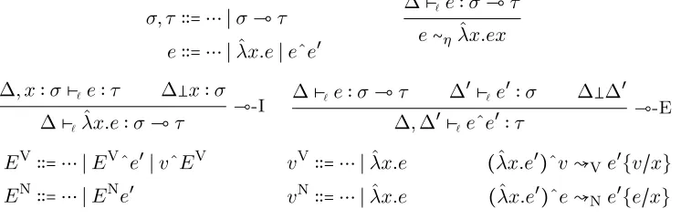
Linear functions. The type of linear functions is written σ⊸τ. Figure 2.1 summarizes the syntax, typing rules, and operational semantics of linear functions. The typing rules for
abstraction ˆλ.e and application eˆe′ ensure that the resources used to produce a function
and its argument are disjoint. The β and η rules are identical to those of the simply-typed
lambda calculus. A lambda closure ˆλx.e is a value in both the name and
call-by-value fragments, but call-by-call-by-value evaluation contexts evaluate the argument to a function
before taking aβ-step. Theη-equivalence rule says that every linear functioneis equivalent
to ˆλx.eˆx.
Multiplicative product. The multiplicative product, also called tensor product and written⊗, is linear in the sense that the two components of the pair cannot use any shared
resources. The fragment of the type system with the multiplicative product is shown in
Figure 2.2.
Unlike the non-linear/Cartesian product, the multiplicative product cannot be
elimi-nated using projections πi ∶σ1⊗σ2 ⊸σi, because such a projection uses only half of the
σ, τ ∶∶= ⋯ ∣σ⊗τ
e∶∶= ⋯ ∣ (e1, e2) ∣let(x1, x2) ∶=ein e′
∆⊢`e∶σ1⊗σ2 ∆′, x∶σ1⊗σ2⊢`e′∶τ ∆∆′ e′{e/x} ∼η let(x1, x2) ∶=ein e′{(x1, x2)/x}
∆1⊢`e1∶σ1 ∆2⊢`e2∶σ2 ∆1∆2 ∆1,∆2 ⊢`(e1, e2) ∶σ1⊗σ2
⊗-I
∆⊢`e∶σ1⊗σ2 ∆′, x1 ∶σ1, x2∶σ2⊢` e′∶τ ∆∆′ ∆,∆′⊢`let (x1, x2) ∶=eine′∶τ
⊗-E
EV∶∶= ⋯ ∣ (EV, e2) ∣ (v1, EV) ∣let (x1, x2) ∶=EVin e′
EN∶∶= ⋯ ∣let(x1, x2) ∶=EN ine′
vV∶∶= ⋯ ∣ (vV1, vV2)
vN∶∶= ⋯ ∣ (e1, e2)
let (x1, x2) ∶= (v1, v2) ine′↝Ve′{v1/x1, v2/x2}
let(x1, x2) ∶= (e1, e2) ine′↝Ne′{e1/x1, e2/x2}
Figure 2.2: Multiplicative product ⊗
letbinding, writtenlet(x1, x2) ∶=eine′, where the two components of the pair are bound
to variables x1 and x2.
Theη-equivalence rule says that, ifeis an expression of typeσ1⊗σ2that occurs linearly
in a larger term e′, thene′{e/x} is equivalent to let(x1, x2) ∶=e in e′{(x1, x2)/x}. That
is, a letbinding can always be commuted to the front of a term.
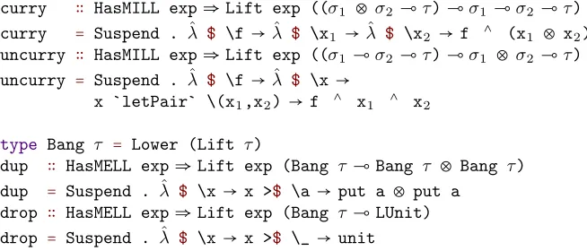
Linear functions can be curried and uncurried with respect to the multiplicative product:
curry∶ (σ1⊗σ2⊸τ) ⊸σ1⊸σ2⊸τ
curry≡λf.ˆ λxˆ 1.λxˆ 2.f(x1, x2)
uncurry∶ (σ1⊸σ2 ⊸τ) ⊸σ1⊗σ2⊸τ
uncurry≡λf.ˆ ˆλx.let(x1, x2) ∶=x in f x1 x2
Multiplicative unit. The multiplicative unit is written LUnitor sometimes 1; the frag-ment corresponding to this type is shown in Figure 2.4. Notice that the call-by-value and
call-by-name rules are identical. LUnitis a unit of ⊗ in the sense thatLUnit⊗σ (and also
lunit⊗○lunit′⊗∼ηλz.lunitˆ ⊗(lunit′⊗ z) ∼βλz.ˆ (lunit′⊗ z,())
∼βλz.ˆ (let(x, y) ∶=z in let () ∶=y in x,()) ∼ηλz.letˆ (x, y) ∶=z in(let() ∶=y in x,()) ∼ηλz.letˆ (x, y) ∶=z in let () ∶=y in(x,()) ∼ηλz.letˆ (x, y) ∶=z in(x, y)
∼ηλz.zˆ
lunit⊗′ ○lunit⊗∼ηλx.lunitˆ ′⊗(lunit⊗x) ∼βλx.lunitˆ ′⊗(x,())
∼βλx.letˆ (x, y) ∶= (x,()) in let () ∶=y inx ∼βλx.letˆ () ∶= ()in x
∼βλx.xˆ
Figure 2.3: Proof thatLUnit is the unit of⊗.
to the identity:
lunit⊗∶σ⊸σ⊗LUnit
lunit⊗≡ˆλx.(x,())
lunit′⊗∶σ⊗LUnit⊸σ
lunit′⊗≡λz.letˆ (x, y) ∶=z in let () ∶=y in x
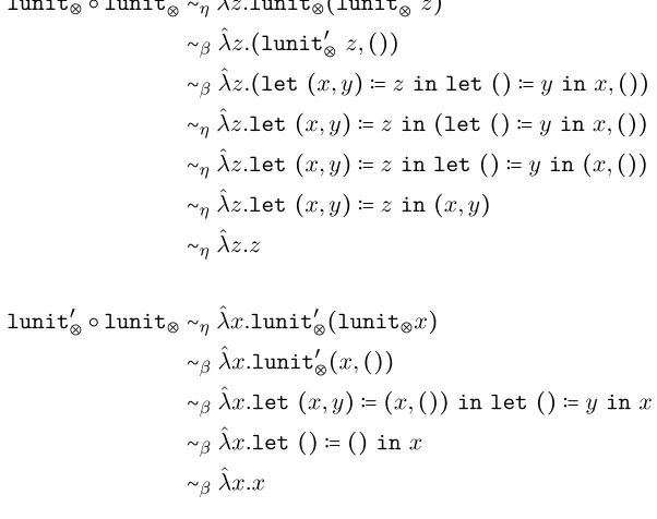
The proofs thatlunit⊗○lunit′⊗ and lunit′⊗○lunit⊗ are identity functions are shown in
Figure 2.3.
The definition oflunit′⊗ here is overly verbose; informally we write ˆλ(x,()).x.
Additive product. Linear type systems often contain two different sorts of products. The additive product, written σ&τ and pronounced “σ withτ,” corresponds more closely
with the non-linear/Cartesian product. Given a computationeof typeσ1&σ2, the user can
choose to use the first component or the second component, but not both, via projection.
This means that to construct an additive pair, the two components of the pair, [e1, e2],
must use exactly the same resources. Intuitively, a computation of type σ1&σ2 provides a
σ, τ ∶∶= ⋯ ∣LUnit
e∶∶= ⋯ ∣ () ∣let () ∶=ein e′
∆⊢`e∶LUnit ∆′⊢`e′∶τ ∆∆′ e′{e/x} ∼η let() ∶=ein e′{()/x}
∅ ⊢`() ∶LUnit
LUnit-I
∆⊢`e∶LUnit ∆′⊢`e′∶τ ∆∆′ ∆,∆′⊢`let() ∶=ein e′∶τ
LUnit-E
EV∶∶= ⋯ ∣let () ∶=EV ine′ EN∶∶= ⋯ ∣let () ∶=EN ine′
vV∶∶= ⋯ ∣ ()
vN∶∶= ⋯ ∣ ()
let() ∶= () ine′↝Ve′
let() ∶= () ine′↝Ne′
Figure 2.4: Multiplicative unitLUnit
σ, τ ∶∶= ⋯ ∣σ&τ
e∶∶= ⋯ ∣ [e1, e2] ∣π1e∣π2e
vV, vN∶∶= ⋯ ∣ [e1, e2]
∆⊢` e∶σ1&σ2
e∼η[π1e, π2e]
∆⊢`e1∶σ1 ∆⊢`e2 ∶σ2 ∆1∆2
∆⊢`(e1, e2) ∶σ1&σ2
&-I
∆⊢`e∶σ1&σ2
∆⊢`π1e∶σ1
&-E1
∆⊢`e∶σ1&σ2
∆⊢`π2e∶σ2
&-E2
EV∶∶= ⋯ ∣πiEV
EN∶∶= ⋯ ∣πiEN
vV∶∶= ⋯ ∣ [e1, e2]
vN∶∶= ⋯ ∣ [e1, e2]
πi[e1, e2] ↝Vei
πi[e1, e2] ↝Nei
Figure 2.5: Additive product
not be evaluated until a choice is made. The typing and evaluation rules for the additive
product are shown in Figure 2.5.
The unit of the additive product, LTop, can be interpreted as a computation throwing
an error. Its rules are shown in Figure 2.6. The error computation is valid under any
σ, τ ∶∶= ⋯ ∣LTop e∶∶= ⋯ ∣error
∆⊢` e∶LTop e∼η error
∆⊢`error∶LTop
LTop-I vV, vN∶∶= ⋯ ∣error
Figure 2.6: Additive unit: LTop
σ, τ ∶∶= ⋯ ∣σ⊕τ
e∶∶= ⋯ ∣ι1e∣ι2e∣caseeof (ι1x1→e1∣ι2x2→e2)
∆⊢` e∶σ1⊕σ2 ∆′, x∶σ1⊕σ2 ⊢`e′∶τ
e′{e/x} ∼η case eof(ι1x1→e′{ι1x1/x} ∣ι2x2→e′{ι2x2/x})
∆1⊢` e1∶σ1
∆1,∆2⊢`ι1∶σ1⊕σ2 ⊕-I1
∆1⊢`e2∶σ2
∆1,∆2 ⊢`ι2∶σ1⊕σ2 ⊕-I2
∆⊢`e∶σ1⊕σ2 ∆′, x1∶σ1⊢`e1∶τ ∆′, x2∶σ2⊢`e2 ∶τ ∆∆′
∆,∆′⊢`case eof (ι1x1→e1∣ι2x2→e2) ∶τ
⊕-E
EV∶∶= ⋯ ∣ιiEV∣caseEV of (ι1x1→e1∣ι2x2→e2)
EN∶∶= ⋯ ∣caseEN of (ι1x1→e1∣ι2x2→e2)
vV∶∶= ⋯ ∣ιivV
vN∶∶= ⋯ ∣ιie
caseιivi of(ι1x1→e1∣ι2x2→e2) ↝Vei{vi/xi} case ιiei of(ι1x1→e1∣ι2x2→e2) ↝Nei{ei/xi}
Figure 2.7: Additive sum
elimination form forLTop. Even so,LTop&σ is isomorphic toσ.
lunit&∶σ⊸σ<op
lunit&≡λx.ˆ [x,error]
lunit′&∶σ<op⊸σ
lunit′&≡ˆλx.π1x
There are no β rules for LTop, but there is an η equivalence: every computation of type
LTop is equivalent to the error computation error.
Additive sum. A computation of type σ ⊕τ is either a computation of type σ or a computation of typeτ; unlike the additive product, the introduction rules dictate which of
σ orτ to provide. To eliminate a sum type, a user must be prepared to accept either result
σ, τ ∶∶= ⋯ ∣LZero e∶∶= ⋯ ∣case eof ()
∆⊢` e∶LZero ∆′, x∶LZero⊢e′∶τ ∆∆′ e′{e/x} ∼ηcase eof ()
∆⊢`e∶LZero ∆∆′ ∆,∆′⊢` case eof() ∶τ
LZero-E
EV∶∶= ⋯ ∣case EV of() EN∶∶= ⋯ ∣case EN of()
Figure 2.8: Additive unit: LZero
The unit of ⊕ is the linear void type, written LZero and shown in Figure 2.8. Like
the non-linear void type, there are no constructors of type LZero, and having a term of
type LZero is a contradiction, so it can be used to derive any type. In particular, given
a computation ∆ ⊢` e ∶ LZero, the computation case e of () can be given any type τ.
Furthermore,case eof ()vacuously uses resources not used by eitself.
lunit⊕∶σ⊸σ⊕LZero
lunit⊕≡ˆλx.ι1x
lunit′⊕∶σ⊕LZero⊸σ
lunit′⊕≡λz.caseˆ zof (ι1x→x∣ι2y→casey of ())
2.3
The exponential modality
!
As we argued in the introduction, it is not enough to just have linear resources; many
domains naturally mix linear resources with non-linear, unrestricted data. Traditionally,
linear logic accounts for unrestricted data with the ! modality (pronounced “bang”). Unlike
with linear resources, itis possible to duplicate and discard unrestricted data.
duplicate∶!σ⊸!σ⊗!σ discard∶!σ⊸LUnit
One interpretation of the ! modality says that an expression of type !σ can be thought of
as a suspended computation that can be executed an arbitrary number of times.
The treatment of ! is one of the most important and delicate components in the design
of a linear type system. It is important because the use of ! affects the usability of the linear
simple butunsound version of !, originally popularized by Abramsky (1993).
Consider a linear computation ∅ ⊢` e∶σ that does not use any linear resources. This
computation can be executed an arbitrary number of times, because each execution does
not use up any resources. We denote such a suspended computation as ∅ ⊢` !e ∶!σ; this
operation is calledpromotion.
More generally, if x1 ∶ !σ1, . . . , xn ∶ !σn ⊢ e ∶ τ uses resources that can themselves be
duplicated, then e can be promoted. Every time e is executed, it will use up one copy
of each of its duplicable resources. Forcing the suspended computation !e executes the
underlying computation, and is calleddereliction.
!∆⊢` e∶σ
!∆⊢`!e∶!σ
promotion
∆⊢`e∶!σ
∆⊢`derelict e∶σ
dereliction
Here, we write !∆ to refer to a context of the form x1∶!σ1, . . . , xn∶!σn
Unrestricted resources are implicitly subject to the structural rules disallowed for plain
linear types—unrestricted resources can be duplicated (also calledcontraction) and dropped
(also called weakening).
∆′, x∶!σ, y∶!σ⊢` e′∶τ
∆, z∶!σ,∆′⊢`e′{z/x, z/y} ∶τ
contraction
∆,∆′⊢`e∶τ
∆, x∶!σ,∆′⊢`e∶τ
weakening
Since we expect suspended computations of the form !e to be evaluated many times,
every suspended computation is a value, and we should never evaluate under a !. The β
rule says that applying dereliction to a promoted expression !eactually executese.
EV∶∶= ⋯ ∣derelictEV
EN∶∶= ⋯ ∣derelictEN
vV∶∶= ⋯ ∣!e
vN∶∶= ⋯ ∣!e
derelict(!e) ↝Ve
Theηrule for !σsays that every computation of !σis equivalent to a suspended computation.
∆⊢`e∶!σ
e∼η !(derelicte)
A refinement of !. Abramsky’s syntax above gives a good first approximation of !, and closely corresponds to Girard’s original presentation as a logical system. However,
Abramsky’s syntax has two serious problems.
First, Abramsky’s syntax is inconsistent with the substitution property (Wadler, 1992).
Consider ∆ ⊢ e ∶ !σ where ∆ may not necessarily have the form !∆—for example, x ∶
LUnit⊢let() ∶=x in !() ∶!LUnit. In addition, notice that a variable y of type !LUnit can
be promoted to !y∶!!LUnit. However, the result of substituting let () ∶=x in !()for y in
!y isnot well-typed:
x∶LUnit /⊢` !(let() ∶=x in !()) ∶!!LUnit
Benton et al. (1993) presented a variation of Abramsky’s syntax that solves the
substi-tution problem and soon became standard. The main difference from Abramsky’s syntax
is that Benton et al.’s syntax requires promotion to explicitly capture all the unrestricted
resources being used.
∆i⊢ei∶!σi x1∶!σ1, . . . , xn∶!σ2⊢e∶τ
∆1, . . . ,∆n⊢promote {ei as xi} ine∶!τ
(Benton et al., 1993)
Bentonet al.’s presentation restores the substitution principle by baking it into the
promo-tion rule.
The second problem with both Abramsky’s and also Benton et al.’s presentations is
practical—it is inefficient and inconvenient to keep explicitly discarding and duplicating
variables via the weakening and contraction rules. There must be a better way to program
Over the years, many styles have been proposed to deal with the problem of linear
syntax, and the remainder of this chapter will highlight four of the most popular. For each,
we also consider how well it models anembedded linear type system—whether an embedded
presentation could use host-language data, libraries, and other tools for non-linear resources,
instead of relying entirely on the embedding for manipulating non-linear data.
2.4
Dual Intuitionistic Linear Logic
Barber’s Dual Intuitionistic Linear Logic (DILL) (1996) is based on the philosophy that
linear and non-linear resources should be treated differently from each other. DILL’s typing
judgment has the form Θ; ∆⊢De∶σ, where σ is a linear type, and Θ and ∆ are both typing
contexts. Resources in Θ (on the left-hand-side of the semi-colon) are unrestricted in e,
while resources in ∆ are linear ine.
Since variables can be either linear or unrestricted, there are two ways to use variables
in DILL. For a linear variable, it is not necessary to limit or keep track of the unrestricted
resources, and for an unrestricted variable, it suffices to check there are no other linear
resources.
x∶σ∈Θ
Θ;∅ ⊢Dx∶σ
DILL-nl-var
Θ;x∶σ⊢Dx∶σ
DILL-l-var
A suspended computation is one that uses no linear resources.
Θ;∅ ⊢De∶σ
Θ;∅ ⊢D!e∶!σ
DILL-!-I
The elimination rule for ! allows the result of a suspended computation to be bound to an
unrestricted variable.
Θ; ∆1⊢De∶!σ Θ, x∶σ; ∆2⊢De′∶τ ∆1∆2
Θ; ∆1,∆2⊢Dlet!x∶=ein e′∶τ
Notice that the same unrestricted resources can be used in both e and e′, even though
their linear resources must be disjoint. This, combined with the intrinsic weakening of the
unrestricted context Θ in the variable rules, means that the weakening and contraction
structural rules need not be included explicitly; they can be derived from the remaining
laws.
In fact, all of Abramsky’s rules are derivable in this system. For example, Abramsky’s
dereliction operator can be derived as follows:
Θ; ∆⊢De∶!σ
Θ; ∆⊢Dderelict e∶σ ≡
Θ; ∆⊢De∶!σ Θ, x∶σ;∅ ⊢Dx∶σ
Θ; ∆⊢D let!x∶=ein x∶σ
The other rules for implication, pairs, and sums are all relatively straightforward. For
example, the rules for linear functions introduce linear variables:
Θ; ∆, x∶σ⊢De∶τ
Θ; ∆⊢Dˆλx.e∶σ⊸τ
DILL-⊸-I
Θ; ∆1⊢De∶σ⊸τ Θ; ∆2⊢De′∶σ
Θ; ∆1,∆2⊢Dee′∶τ
DILL-⊸-E
Alternatively, it’s possible to derive syntax for non-linear functions: let us write σ→τ
for the type !σ⊸τ. We can derive an introduction rule that introduces the argument into
the non-linear context:
Θ, x∶σ; ∆⊢De∶τ
Θ; ∆⊢Dλ!x.eˆ ∶σ→τ ≡
Θ;z∶!σ⊢Dz∶!σ Θ, x∶σ; ∆⊢De∶τ
Θ; ∆, z∶!σ⊢Dlet !x∶=z in e∶τ
Θ; ∆⊢Dλz.letˆ !x∶=z in e∶!σ⊸τ
Related work. The inspiration for tracking linear and non-linear resources in different parts of a context started with Girard’s Logic of Unity (LU) (1993), which unifies several
logical fragment has a designated fragment of the context. Wadler (1994) restricted LU to
its intuitionistic and linear fragments and considered it as a sequent-calculus style syntax
for linear logic, but it was Barber’s natural deduction style that caught on.
Embedded DILL. DILL might be the most popular style of linear type system in prac-tice, but how does it fare as a model for embedded linear types? Our goal is for unrestricted
variables in Θ to hold host-language data. This indicates that host types and linear types
should overlap, since linear variables and non-linear variables have the same types in DILL.
So we take LType to be Type, and we allow non-linear data to be embedded in a linear
expression as follows, where LExpD Θ ∆ α is the type of linear expressions:
a∶α
puta∶LExpD Θ∅ α
If linear types are just host-language types, then how do we distinguish linear connectives
from ordinary non-linear connectives? Consider the linear function typeα⊸β, which must
now correspond to a type in the host language. If that type is inhabited—say, if α⊸β is
the normal function type α →β—then the put constructor would violate linearity, as we
would have put(λx.(x, x)) ∶ LExpD Θ ∅ (α ⊸α×α). On the other hand, we would like
put(λx.(x, x)) ∶LExpD Θ∅ (!α⊸α×α).
It is clear that a theory of embedded DILL would require significant changes to its
meta-theory, so we look for another approach.
2.5
Indexed modalities
DILL syntactically separates non-linear variables Θ from linear variables ∆ in its typing
judgment, but one could equally consider a typing judgment that annotated each variable as
uses a single typing context Φ annotated with resource descriptors r:
Φ∶∶= ∅ ∣Φ, x∶rσ r∶∶=0∣1∣ω
The resource 1 stands for linear use,i.e.,the variable is used exactly once in a term, andω
stands for unrestricted use. The resource 0 stands for an unused resource, so ifx does not
appear in Φ, then Φ is equivalent to Φ, x∶0σ.
These resource descriptors form an algebraic structure known as a rig—a riNg without
Negation:
0+r=r+0=r 0⋅r=r⋅0=0 1⋅r=r⋅1=r
In addition, the unrestricted resource absorbs other resources.
1+1=ω ω+r=r+ω=ω ω⋅ω=ω
The first equation says that when a linear resource (denoted with the resource descriptor 1)
is used more than once in a system, then it it is unrestricted in the combined system. With
a different collection of resources, e.g., resources drawn from Z, we could produce a more
refined analysis; we discuss these more below. The second and third equations say that an
unrestricted resource will always remain unrestricted.
We can extend the rig on resources to a semi-module on indexed typing contexts.
(∆1, x∶r1 σ) + (∆2, x∶r2 σ) ≡ (∆1+∆2), x∶r1+r2 σ
r⋅ (Γ, x∶r′ σ) ≡ (r⋅Γ), x∶r⋅r′ σ
The typing judgment has the form Φ ⊢I e ∶ σ. Like in DILL, we want unrestricted
data annotated with ω to have implicit weakening and contraction, which we can obtain
by modifying how contexts are split. Instead of restricting typing rules to disjoint typing
input contexts.
ω⋅Φ, x∶rσ⊢Ix∶σ
i-var
Φ⊢Ie∶σ Φ′, x∶rσ⊢Ie′∶τ
(r⋅Φ) +Φ′⊢Iletx∶=ein e′∶τ
i-let
In the variable rule, all the variables in ω⋅Φ are unrestricted, so they can be implicitly
weakened. In theletrule, the resources Φ used to constructeare scaled by the number of
times x is being used in the result.
The promotion rule says that any linear expression can be promoted, but the resources
in the result are all scaled by ω, since the result could be used any number of times.
Φ⊢Ie∶σ
ω⋅Φ⊢I!e∶!σ
i-!-I
Φ⊢Ie∶!σ
Φ⊢Iderelicte∶σ
i-!-E
Function types can be annotated with the resource corresponding to how many times
the argument is used.
Φ, x∶rσ⊢Ie∶τ
Φ⊢Iλx.eˆ ∶σ→rτ
i-→-I
Φ⊢Ie∶σ→rτ Φ′⊢Ie′∶σ
Φ+r⋅Φ′⊢Iee′∶τ
i-→-E
Related work. Resource annotations have often been extended to different substructural type systems. The style seems to have originated with bounded linear logic (Girard et al.,
1992) annotating the exponential !nwith a numbernrecording the precise number of times
it is used. The type system presented above can easily accommodate exponentials indexed
by arbitrary resources:
Φ⊢Ie∶σ
r⋅Φ⊢I!e∶!rσ
i-!r-I
Φ⊢Ie∶!rσ
Φ⊢Iderelicte∶σ
By including resources corresponding to affine or substructural use, resource annotations
can express substructural typing systems, or coeffects like data flow, liveness analyses, or
differential privacy (Petriceket al., 2014; Brunelet al., 2014; Reed and Pierce, 2010).
McBride (2016) uses resource annotations in a calculus for linear dependent types, where
variables can be used in types with a resource annotation of x ∶0 σ. McBride indexes not
only variables, but also the typing judgment itself, with a resource: Φ⊢Ie∶rσ, which takes
the place of the exponential !r.
Bernardyet al.(2017) use resource annotations in a calculus that retrofits Haskell with
linear types. Their typing judgment, though, has a unique interpretation: the typing
judg-ment Φ⊢e∶σ in their system means that if the result of eis consumed exactly once, then
the linear hypotheses in Φ will be consumed exactly once. However, any top-level expression
can be consumed multiple times, to make the calculus backwards-compatible and facilitate
code reuse between linear and non-linear types. This means that if a program wants to
guarantee linear use of a piece of data, it must bind that data on the left-hand-side of a
function type, as in σ→1τ. In practice this seems to result in a style of programming akin
to continuation-passing style.
Embedded indexed modalities. Like DILL, the presentation in terms of indexed modal-ities requires that both linear and non-linear resources share the same kind of type. But
now we can define the type α→rβ as a wrapper for α→β when r is ω, and otherwise as
an empty type.
data α→r β where
fun : (α→β)→ (α→ω β)
Thus, non-linear functionsf ∶α→β can be coerced into a linear expressionput(funf) of
linear type α→ω β, but not into the type α→1 β, which can only be constructed via the
embedded ˆλconstructor.
e∶LExpI (Φ, x∶rα) β
ˆ
λx.e∶LExpI Φ(α→rβ)
e∶LExpI Φ (α→rβ) e
′∶LExp
I Φ
′ α
eˆe′∶LExpI (Φ+r⋅Φ
Non-linear functions from host-language libraries can now be applied to linear arguments.
For example, consider thelookupoperation from the linear interface to mutable references
discussed in Chapter 1.
lookup∶LExpI (ω⋅Φ) (LRef α→1α⊗LRef α)
We can lift arbitrary functions of type α→β to the result oflookup:
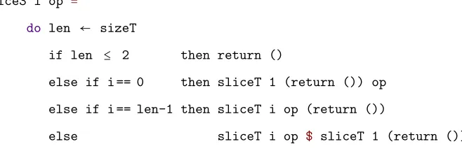
op∶ (α→β) →LExpI (ω⋅Φ) (LRefα→1β⊗LRef α)
op≡λf.ˆλr.let(x, r′) ∶=lookupr in (putfˆx, r′)
But what is the operational semantics ofput? Is(putf)a value? If so, then isput fˆ v
a stuck term? What about put f ˆ put a?
These questions may not be insurmountable, but they are not straightforward from the
theory of indexed resource modalities.
2.6
Kind-based linear logic
The previous two presentations assume that, while linear and non-linear variables should
be treated differently, all types are inherently the same. Kind-based presentations of linear
logic suggest that linear data is inherently different from non-linear data, and the type
system should distinguish them.
System F○ (pronounced “F-pop”), introduced by Mazurak et al. (2010), has a kind ∗
allows type variables and quantification over type variables X.
Φ⊢Kσ∶ ∗
Φ⊢Kσ∶ ○
sub
Φ⊢Kσ1∶κ1 Φ⊢Kσ2∶κ2
Φ⊢Kσ1
κ Ð→σ2∶κ
→
X∶κ∈Φ
Φ⊢KX∶κ
tvar
Φ, X∶κ1⊢Kσ∶κ2
Φ⊢K∀X∶k1. σ∶k2 ∀
In the first rule, non-linear types can be coerced into linear types. In the second rule, a
function depends on three parameters: the kind of its argument; the kind of its result;
and the kind of the function itself, which annotates the top of the arrow. For example,
the linear identity type may be given the type σ Ð→∗ σ for ⊢K σ ∶ ○, because although the
function uses its argument linearly, the function itself is linearly closed, and so can be used
arbitrarily many times. So, although System F○ doesn’t include a ! operator on types, it
can be approximated as !σ ≡Unit Ð→∗ σ ∶ ∗, where Unit ∶ ∗ is a non-linear unit type, and
σ∶ ○ is a linear type.
Typing contexts can either be separated according to the kind of the type being stored,
as in DILL, or they can be combined as in the resource-annotated calculi. We choose the
latter presentation, and we again write Φ1+Φ2 for the linear merge of contexts Φ1 and Φ2.
The subkinding relation can be written as a reflexive, transitive relationκ1≥κ2, with∗ ≥ ○.
This relation can be extended to contexts Φ≥ κ to say that every type in Φ has kind κ′
such thatκ′≥κ.
Φ≥ ∗
Φ, x∶σ⊢Ke∶σ
F○-var
Φ, x∶σ⊢Ke∶τ Φ≥κ
Φ⊢Kλx.eˆ ∶σ
κ Ð→τ
F○-→-I
Φ1⊢Ke∶σ
κ
Ð→τ Φ2⊢Ke′∶σ
Φ1+Φ2⊢Keˆe′∶τ
Related work. Later calculi including Alms (Tov and Pucella, 2011) and Quill (Morris, 2016) present variations of System F○ with the addition of kind polymorphism and more
nuanced subkinding. For example, in Alms (which is actually an affine type system), the
identity function can be given the type ∀κ,∀(σ ∶κ), σ Ð→∗ σ. This makes it easier to reuse
code and means that every well-typed program has a single most general type. However,
the presentation of that most general type can be quite complex.
For example, in plain System F○, the expression ˆλx. ˆλy. x, which discards its second
argument, can be given one of four types:
∀(X∶ ○)(Y ∶ ∗), XÐ→∗ Y Ð→○ X ∀(X∶ ○)(Y ∶ ∗), XÐ→○ Y Ð→○ X
∀(X∶ ∗)(Y ∶ ∗), XÐ→∗ Y Ð→∗ X ∀(X∶ ∗)(Y ∶ ∗), XÐ→○ Y Ð→∗ X
In Alms, however, this argument can be given a single most general type:
∀(X∶κ)(Y ∶ ∗), XÐ→∗ Y Ð→k X (2.1)
The four types above are all subtypes of Equation (2.1).
Embedded System F○. An embedded version of System F○ would have its types of kind ∗ overlap with host-language types, but types of kind ○ be distinct. Let Kind be a
type with two constructors, ○ and ∗, and define Pop : Type to be a data kind of linear
types. Then we can define J−K∶Kind→Typeso that J○K=Pop:
data Pop where
Var : Nat → Pop
Sub : Type → Pop
PopArrow : Π {κ1 κ2 : Kind}, Jκ1K → Jκ2K → Pop
data Kind where
∗ : Kind ○ : Kind
J∗K ≡ Pop
The linear type Sub α : Pop corresponds to the subkinding rule sub. The linear type
PopArrow σ1 σ2 corresponds only to σ1 Ð→○ σ2, as σ1 Ð→∗ σ2 must be a host-language type.
In particular, ifσ1 and σ2 both have kind∗, thenσ1Ð→∗ σ2 should correspond to the regular
host-language function type σ1→σ2. However, if either σ1 orσ2 has kind○, then the type
should be uninhabited.
data StarArrow : Π (κ1 κ2 : Kind), Jκ1K → Jκ2K → Type where
Arrow : Π (α β : Type), (α→β)→ StarArrow α β
If made explicit, the subkinding relation from ∗ to ○could give some indication about
the behavior of put, which injects host-language data into the linear embedded language.
For example, we might expect host data a ∶α can be embedded into put a of ∗-type α,
which can then be coerced to a linear typeSub α.
a∶α Φ≥ ∗
puta∶LExpK Φα
e∶LExpK Φα
e∶LExpK Φ(Sub α)
The subtyping relation should further coerce the type Sub (StarArrow σ1 σ2) into
PopArrow σ1 σ2 so that put(Arrow f)ˆput a reduces to put(f a). But this doesn’t fully
explain the semantics ofput—what if the argument toput Arrowf does not have the form
puta?
System F○’s subkinding relation is implicit, but in an embedded language the two kinds
would be explicit; thus F○’s meta-theory does not characterize a linear embedding.
2.7
Linear/non-linear logic
Introduced by Benton (1995) and illustrated in Figure 2.9, linear/non-linear (LNL) logic
makes a distinction between the syntax of linear and non-linear types, whereas System F○
distinguishes them via a kinding judgment. Linear types, which we continue to denote with
the meta-variableσ, are distinguished from non-linear types, which we denoteα. The LNL
system similarly consists of two kinds of variables (linearxand non-lineara), and two kinds
linear fragment non-linear
fragment
⊣ Lift
Lower
Figure 2.9: The linear/non-linear categorical model. The model consists of two categories related by functors Lift and Lower that form a categorical adjunction Lift⊣Lower; for details see Section 5.3.
two kinds of terms, depending on whether the result is a linear or non-linear type.
A linear expressionecan be thought of as a computation that consumes linear resources
and also has access to non-linear variables. Its typing judgment is written Γ; ∆ ⊢B e ∶ σ,
where ∆ is a linear typing context and Γ is a non-linear typing context.1 A non-linear
term t cannot access any linear resources, so it can be thought of as a value instead of a
computation. The typing judgment for non-linear data has the form Γ⊢Bt∶α, where it only
has access to non-linear variables. From these two typing judgments, there are two variable
rules and three let bindings: non-linear variables bound in a non-linear term; non-linear
variables bound in a linear term; and linear variables bound in a linear term.
Γ;x∶σ⊢Bx∶σ
LNL-`-var
a∶α∈Γ
Γ⊢Ba∶α
LNL-n`-var
Γ; ∆⊢Be∶σ Γ; ∆′, x∶σ⊢Be′∶τ ∆∆′
Γ; ∆,∆′⊢Bletx∶=ein e′∶τ
LNL-let-`-in-`
Γ⊢Bt∶α Γ, a∶α; ∆⊢Be∶τ
Γ; ∆⊢Bleta∶=t ine∶τ
LNL-let-n`-`
Γ⊢Bt∶α Γ, a∶α⊢Bt′∶β
Γ⊢Bleta∶=tin t′∶β
LNL-let-n`-n`
1
α∶∶= ⋯ ∣Lift σ t∶∶= ⋯ ∣suspende e∶∶= ⋯ ∣forcet
Γ⊢Bt∶Liftσ
t∼η suspend(force t)
Γ;∅ ⊢Be∶σ
Γ⊢Bsuspend e∶Lift σ
Lift-I Γ⊢Bt∶Lift σ Γ;∅ ⊢Bforce t∶σ
Lift-E
EV∶∶= ⋯ ∣forceEV EN∶∶= ⋯ ∣forceEN
vV∶∶= ⋯ ∣suspend e vN∶∶= ⋯ ∣suspend e
force(suspend e) ↝Ve
force(suspend e) ↝Ne
Figure 2.10: LNL Lift connective
Because there are both linear and non-linear types and terms, there must be two sorts
of every connective—two kinds of products, two kinds of functions, etc.. The non-linear
product, for example, is only relevant in the non-linear typing judgment, and conversely for
the linear products.
Γ⊢Bt1∶α1 Γ⊢Bt2∶α2
Γ⊢B(t1, t2) ∶α1×α2
LNL-×-I
Γ⊢Bt∶α1×α2
Γ⊢Bπit∶αi
LNL-×-E
Γ; ∆1⊢Be1∶σ1 Γ; ∆2⊢Be2∶σ2 ∆1∆2
Γ; ∆1,∆2⊢B(e1, e2) ∶σ1⊗σ2
LNL-⊗-I
Γ; ∆⊢Be∶σ1⊗σ2 Γ; ∆′, x1∶σ1, x2∶σ2⊢Be′∶τ ∆∆′
Γ; ∆,∆′⊢Blet(x1, x2) ∶=ein e′∶τ
LNL-⊗-E
The exponential operator ! is broken up into two parts in LNL, as illustrated in
Fig-ure 2.9.
The first operator takes a linear type σ and lifts it to a non-linear type, Lift σ,
sum-marized in Figure 2.10. The introduction and elimination rules forLift correspond to the
promotion and dereliction rules for !, which we write in this case as suspend and force.
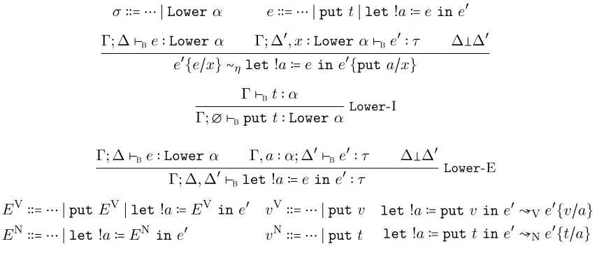
σ∶∶= ⋯ ∣Lowerα e∶∶= ⋯ ∣putt∣let!a∶=ein e′
Γ; ∆⊢Be∶Lowerα Γ; ∆′, x∶Lower α⊢Be′∶τ ∆∆′
e′{e/x} ∼η let!a∶=eine′{puta/x}
Γ⊢Bt∶α
Γ;∅ ⊢Bputt∶Lower α
Lower-I
Γ; ∆⊢Be∶Lowerα Γ, a∶α; ∆′⊢Be′∶τ ∆∆′
Γ; ∆,∆′⊢Blet !a∶=ein e′∶τ
Lower-E
EV∶∶= ⋯ ∣putEV∣let!a∶=EV ine′ EN∶∶= ⋯ ∣let!a∶=EN ine′
vV∶∶= ⋯ ∣putv vN∶∶= ⋯ ∣putt
let!a∶=putv in e′↝Ve′{v/a}
let !a∶=put tin e′↝Ne′{t/a}
Figure 2.11: LNL Lowerconnective
The second operator takes a non-linear type α to a linear type Lower α, as shown in
Figure 2.11. Any host-language termtof typeα can be coerced into a (linear) computation
put t of type Lower α that returns the value of t. A computation of type Lower α can
be bound to a non-linear variable a, so that the result can be used non-linearly in the
continuation.
The original ! modality can be derived from the composition ofLower and Lift:
Γ;∅ ⊢Be∶σ
Γ;∅ ⊢B!e∶!σ ≡
Γ;∅ ⊢Be∶σ
Γ⊢Bsuspend e∶Lift σ
Γ;∅ ⊢Bput(suspend e) ∶Lower(Lift σ)
Γ; ∆⊢Be∶!σ
Γ; ∆⊢Bderelicte∶σ ≡
Γ; ∆⊢Be∶Lower(Liftσ)
Γ, a∶Lift σ⊢Ba∶Lift σ
Γ, a∶Lift σ;∅ ⊢Bforce a∶σ
Γ; ∆⊢Blet !a∶=ein force a∶σ
Related work. The idea of having separate typing judgments for different kinds of types is closely related to Levy’s call-by-push-value (CBPV), which makes the distinction between