Image-Processing Software for High-Throughput Quantification of Colony Luminescence

Image-Processing Software for High-Throughput

Quantification of Colony Luminescence

Eyal Dafni,

_{Iddo Weiner,}

_{Noam Shahar,}

_{Tamir Tuller,}

_{Iftach Yacoby}

a_{School of Plant Sciences and Food Security, The George S. Wise Faculty of Life Sciences, Tel Aviv University, Tel Aviv, Israel}

b_{Department of Biomedical Engineering, The Iby and Aladar Fleischman Faculty of Engineering, Tel Aviv University, Tel Aviv, Israel}

c_{The Sagol School of Neuroscience, Tel Aviv University, Tel Aviv, Israel}

ABSTRACT

Many microbiological assays include colonies that produce a

lumines-cent or fluoreslumines-cent (here generalized as “lumineslumines-cent”) signal, often in the form of

luminescent halos around the colonies. These signals are used as reporters for a trait

of interest; therefore, exact measurements of the luminescence are often desired.

However, there is currently a lack of high-throughput methods for analyzing these

assays, as common automatic image analysis tools are unsuitable for identifying

these halos in the presence of the inherent biological noise. In this work, we have

developed CFQuant—automatic, high-throughput software for the analysis of

im-ages from colony luminescence assays. CFQuant overcomes the problems of

auto-matic identification by relying on the luminescence halo’s expected shape and

pro-vides measurements of several features of the colonies and halos. We examined the

performance of CFQuant using one such colony luminescence assay, where we

achieved a high correlation (

R

⫽

0.85) between the measurements of CFQuant and

known protein expression levels. This demonstrates CFQuant’s potential as a fast

and reliable tool for analysis of colony luminescence assays.

IMPORTANCE

Luminescent markers are widely used as reporters for various

biologi-cally interesting traits. In colony luminescence assays, the levels of luminescence

around each colony can be used to compare the levels of traits of interest for

differ-ent strains, treatmdiffer-ents, etc., using quantitative measuremdiffer-ents of the luminescence.

However, automatic methods of obtaining this data are underdeveloped, making

this a laborious manual process, especially in analyzing large numbers of colonies.

The significance of this work is in developing an automatic, high-throughput tool for

quantitative analysis of colony luminescence assays, which will allow fast collection

of qualitative data from these assays and thus increase their overall usability.

KEYWORDS

fluorescent-image analysis, microbial method, software

L

uminescent and fluorescent reporters (here generalized as “luminescent” reporters

[1]) are widely used in all fields of biological research (2–5). As research progresses,

the scale of experiments is growing and the need for high-throughput quantitative

analyses from a large set of luminescence-based assays is rising accordingly (6).

The analysis of colony luminescence is a major step in various assays; in such setups,

colonies typically express a luminescent marker (e.g., green fluorescent protein [GFP],

luciferase, mCherry, etc.) which is used to verify transformation (7–9), report on gene

expression (10–13), report on cellular localization (14–16), indicate binding between

entities (17–19), or monitor growth rates (20–22) or for any other purpose. In these

types of assays, the output usually consists of a pair of images: (i) an image displaying

the plated microbe or cell colonies and (ii) an image of the same plate taken with a

relevant camera and exhibiting various levels of colony luminescence. The typical task

CitationDafni E, Weiner I, Shahar N, Tuller T, Yacoby I. 2019. Image-processing software for high-throughput quantification of colony luminescence. mSphere 4:e00676-18.https:// doi.org/10.1128/mSphere.00676-18.

EditorCraig D. Ellermeier, University of Iowa

Copyright© 2019 Dafni et al. This is an open-access article distributed under the terms of theCreative Commons Attribution 4.0 International license.

Address correspondence to Tamir Tuller, [email protected], or Iftach Yacoby, [email protected].

E.D. and I.W. contributed equally to this article.

Received6 December 2018

Accepted7 December 2018

Published2 January 2019

Applied and Environmental Science

crossm

on September 8, 2020 by guest

http://msphere.asm.org/

is that of quantifying the probed trait from the luminescence image while normalizing

the signal by the size of the colonies, as deduced from the first image.

Current technologies for large-scale accurate quantification of these images are

underdeveloped. The reason for this gap in relevant analysis tools lies in the inherent

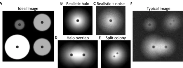
noise of these biological assays. While a theoretical plate (Fig. 1A) could be analyzed

with common image-processing tools (e.g., the ImageJ [23] user interface or similar

tools), images obtained from real experiments contain artifacts which hinder the ability

of general image-processing algorithms to properly analyze them. The most common

artifacts are soft edges of the luminescent halos (Fig. 1B), image noise (Fig. 1C), halo

overlaps (Fig. 1D), and split colonies (Fig. 1E). If general image-processing tools are

used, quantitative analysis of images with combinations of all these artifacts (Fig. 1F)

requires heavy user input. Thus, researchers interested in accurate quantification of

their assay often have to (i) adjust the contrast until a threshold that seems right

according to their perception is found, (ii) manually mark each halo separately, and (iii)

manually subtract halo intensity data resulting from overlapping regions. The

labori-ousness of this procedure drives researchers toward either keeping their assays small or

analyzing the results qualitatively.

To address these issues, we developed a general software package—CFQuant—for

analyzing colony luminescence while taking typical levels of biological noise (Fig. 1)

into consideration. As a study case, we used the

Rhodobacter capsulatus

high-throughput screening system (24, 25). In that assay, plates containing algal colonies are

overlaid with engineered bacteria which produce GFP in the presence of gaseous

hydrogen (H2). This system, which generates a luminescence image (GFP) alongside a

colony image (chlorophyll), is typically used as a qualitative phenotypic screen that

reports on desirable genetic traits in heterogeneous populations (25–29). This assay

represents a classical large-scale experiment in which the output is a colony

lumines-cence image with an array of biological noise data which have so far prevented a

quantitative analysis. Using our novel image-processing tool, we show here that we are

able to overcome the noise issues and formulate a sound quantitative prediction of

active-enzyme abundance in each colony on the basis of these large-scale screening

images alone.

CFQuant is available at

https://www.energylabtau.com/cfquant

.

RESULTS

Software details.

Upon initiation of the software, the user is required to upload

the colony and halo images and to choose the colony detection method— either

FIG 1 Illustration of common artifacts in automatic identification of luminescent halos. (A) An ideal image, with clear halo borders. The darker spots in the center of each halo represent the colonies. (B) A more realistic halo, with its values slowly decreasing from the center. This creates soft edges, with very small difference in values between the halo’s edge and the background. (C) As described for panel B, but with the addition of noise, which lessens the difference between the halo and the background even further. (D) Two overlapping halos. Notice that the area of overlap is brighter (i.e., has higher values) than the other side of each halo. (E) A split colony, separated into two areas (indicated by the two dark spots). (F) The common result of a colony luminescence assay: the image is noisy, the halo values are gradually decreasing, and both overlaps and split colonies may exist.

on September 8, 2020 by guest

http://msphere.asm.org/

arrangement-based or scatter-based detection. To use arrangement-based detection,

the user must also upload an approximate arrangement of the colonies in a grid of rows

and columns (see Materials and Methods for image requirements). The user also has the

choice of either analyzing a single image or performing batch processing—analysis of

multiple images—without the user interaction steps.

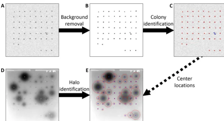
Once the input is received, CFQuant starts analyzing the colony image (Fig. 2A). The

software begins with an initial background removal step, after which the image is left

with several foreground areas (Fig. 2B). However, in some images the number of

foreground areas exceeds the specified number of colonies. In arrangement-based

detection, CFQuant compares the arrangement of the foreground areas with the

user-specified arrangement and determines by this comparison if the excess areas are

due to persisting background noise or cases of split colonies (Fig. 1E) or both. It then

either joins foreground areas that are in close proximity or deletes low-value ones until

no excess areas remain. In scatter-based detection, the colony number is unknown, so

the software uses the shapes, sizes, and values of the foreground areas to ensure that

background noise is deleted. Split-colony identification is not performed using this

method. Regardless of the method chosen, in the final stage the software determines

the background threshold value (i.e., the value below which pixels are considered part

of the background). Once the colonies are identified, the user can view the results and

make changes if necessary (Fig. 2C).

After ensuring that colonies were correctly identified, CFQuant moves on to the halo

image (Fig. 2D). For each halo, the software attempts to find the threshold value

separating it from the background. Since edge detection is problematic in the

lumi-nescent halos (Fig. 1), CFQuant relies on the fact that halos form circular shapes

centered at (or near) the middle of the colony. In cases of halo overlaps (Fig. 1D), each

halo is expected to resemble a partial circle. Therefore, the software first assigns to each

halo the highest possible background threshold value and then gradually decreases it

until the area no longer resembles a circle (or a partial one). The stopping point is

determined based on the distances corresponding to each edge point from the colony

center being roughly equal while still allowing some noise in the distance and center

location. As in the previous phase, once all the halos are identified, the user can view

the results and make changes if necessary (Fig. 2E).

FIG 2 The flow of the software in analyzing a single plate. (A) The colony image of the plate before analysis. (B) The colony image after the background removal step. (C) The colony image after colony identification. The identified colony borders are shown in red. The blue borders mark two areas that were identified as parts of a split colony. (D) The halo image before analysis. Image contrast was adjusted for visibility. (E) The halo image after identification. The identified halo borders are shown in red. The blue dots mark the centers of the colonies, which are used in the halo identification.

on September 8, 2020 by guest

http://msphere.asm.org/

After the analysis is completed, data on both the colonies and the halos are saved.

The saved data include the area, pixel sum, mean pixel value, and maximal pixel value

corresponding to each colony and each halo. The latter three parameters are also

evaluated using normalized calculations based on the selected background thresholds

(see Materials and Methods for more details). In the halo image, pixel values in areas of

overlap are corrected to the values expected for each halo to avoid the additive effect

in the overlap area (Fig. 1D).

Automatic identification test.

Colony identification performed using

arrangement-based detection correctly identified 100% of the colonies on all 31 plates tested (each

plate contained 20 to 109 colonies). Using scatter-based detection on the same plates,

99% of the colonies were correctly identified. In testing performed on plates containing

16 to 656 scattered colonies, 88% of the colonies were correctly identified (83% to 94%

for each plate individually). A total of 60 areas representing background noise were

mistakenly identified as colonies (3% of identified colonies); all were dark spots at the

edge of the plates. Fig. S1 in the supplemental material shows an example of images

identified with scatter-based detection.

Among 695 noticeable halos in all 37 plates, 671 (97%) were identified

automati-cally. However, 13% of them were considerably smaller or larger than their size as

perceived by eye. Twelve colonies (2% of the identified halos) were erroneously given

a halo.

In images with fewer than 200 colonies and sizes of up to 625-by-625 pixels, the

durations of automatic identification were at most 5 s for the colony image and 34 s for

the halo image, using CFQuant from MATLAB version 2017b on Windows 7 (Intel Core

i7 6700; CPU, 3.4 Ghz). It should be noted that the individual images had no more than

36 noticeable halos in them. With the largest colony number (656, only 8 of which had

noticeable halos), automatic identification took 21 s for the colonies and 77 s for the

halos.

Performance test.

To test our software, we performed the

R. capsulatus

assay on

20 engineered strains of

Chlamydomonas reinhardtii

with known expression levels

of a synthetic H

-producing enzyme (29). To produce images for the software, these

strains were plated on four replica plates of 20 clones each. Two images were

obtained for each plate: a colony image and a halo image of the GFP fluorescence.

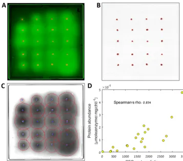
Fig. 3A shows a composite (manually colored and contrasted) image of one of the

plates from this assay. We analyzed these images using CFQuant (Fig. 3B and C

show the identified colonies and halos, respectively, of the plate displayed in

Fig. 3A) and obtained the features (measured values) of each halo and colony. To

control for colony size, we divided the halo feature data by the colony feature data.

We then averaged the results of all four plates and searched for the single feature

that best predicted the known protein abundance (calculated from three

repeti-tions of active-protein quantification; see “MV protein quantification” in Materials

and Methods). Of the 10 halo features, the best predictor was the pixel sum

normalized by each halo’s individual threshold (see Materials and Methods). This

value (divided by the colony area value) had a Spearman’s rho of 0.854 (

P

value

⬍

10

₎

when correlated with the known protein abundance levels (Fig. 3D). To further

validate the performance of CFQuant, we performed a manual analysis of the same

images using ImageJ (23). In measuring a similar normalized pixel sum divided by

the colony area, the correlation of the values with the known protein abundance

had a Spearman’s rho of 0.759 (

P

value

⬍

2

*

10

_{) (Fig. S2). Levels of correlation of}

other values (area, sum, etc.) divided by colony area with the protein abundance

were lower (not shown).

DISCUSSION

In this work, we developed CFQuant—a MATLAB-based image-processing tool built

to meet the needs for a growing practice of using luminescent markers in large-scale

assays. CFQuant is designed as a quick and reliable tool for quantifying colony

lumines-cence while overcoming an array of prevalent forms of biological noise. CFQuant is a

on September 8, 2020 by guest

http://msphere.asm.org/

high-throughput tool. In addition to providing automatic analysis of individual plates,

CFQuant also has a batch-processing mode that allows it to analyze multiple images

with no user interaction. This enables CFQuant to provide fast analyses of very large

numbers of colonies. These qualities allow CFQuant to be a considerably faster

alter-native to manual analysis of images, especially in working with larger assays.

Halo edge detection.

The most fundamental issue that CFQuant had to overcome

was the problem of automatically detecting halos. Most classical edge detection

algorithms (such as are implemented in most generalist image analysis software) look

for a noticeable drop in pixel intensity in order to determine object edges (30).

However, colony luminescence halos tend to be gradual, with soft edges (see Fig. S3A

in the supplemental material), and lack this drop in pixel intensity. In manually

adjusting the contrast, it might appear as if clear edges are present (Fig. S3B), but the

pixels hidden by the contrast settings would still pose a problem for automatic tools.

Therefore, mainstream edge detection methods struggle to define clear halo

bound-aries (Fig. S3C). Permanently changing the image’s pixel values to the manually selected

contrast values could remedy this problem but would do so at the expense of loss of

information from the image.

We tackled this issue in a different way; as CFQuant is a software program optimized

for detecting and quantifying colony luminescence, we used some of the natural traits

of these assays to solve the problems of halo detection. Instead of looking for steep

FIG 3 The results of the performance test. (A) Composite image of one of the plates used in the assay, combining the colony and halo images. The colonies are shown in red, and the GFP halos are shown in green. (B) The colony image after CFQuant analysis. The detected colony borders are shown in red. (C) The halo image after CFQuant analysis. The detected borders of the halos are shown in red, and the colony centers are shown in blue. (D) The best correlation of a single halo feature with the known protein expression values of the strains (Pvalue⬍10⫺5_).

The CFQuant prediction represents the normalized sum of pixels for the halos divided by the area of the colonies, as described in the text. The values used in the figure represent averages of the measurements from all four plates. The protein abundance represents the average of results from three measurements performed with methyl viologen (see “MV protein quantification” in Materials and Methods). chl, chlorophyll.

on September 8, 2020 by guest

http://msphere.asm.org/

decreases in pixel intensity, we exploited the fact that halos are roughly centered

around the colony producing them—and thus, we begin our halo search from the

colony coordinates. From this point, the area analyzed by the software gradually

spreads out in a search for the halo’s edge. Since halation takes on a circular shape by

definition, we can look for radial signals instead of intensity drops; thus, CFQuant is able

to detect halo boundaries properly (Fig. S3D), uniformly and automatically—making it

suitable for large-scale assays. It should be noted that the halo centers are not expected

to be exactly at the location of the colony centers, and thus, our method allows for

some freedom in their alignment (Fig. 3C).

This method also allows CFQuant to overcome another common issue in halo

identification— overlaps. By identifying the partial circle belonging to each of the

overlapping halos, CFQuant is able to estimate the original boundaries of each halo.

These boundaries are later used to avoid overestimating the intensity of overlapping

halos. CFQuant performs well even in assay plates with many overlaps (Fig. 3).

It is worth mentioning that in quantifying images of colony fluorescence from the

R. capsulatus

assay, we achieved better results with CFQuant than were achieved in

measurement of the images manually with ImageJ (Spearman’s rho of 0.854 versus

0.759, respectively, when correlated with the known protein abundance). We believe

this is mostly due to CFQuant’s ability to compensate for the halo overlaps, which were

abundant in our images (Fig. 3C), though it is also possible that the determination of

halo edges was less consistent when working manually.

Using CFQuant.

In this work, we tested the performance of CFQuant on a specific

assay and obtained high levels of correlation with active-protein abundance

measure-ments in using the normalized pixel sum of the halos. However, CFQuant was built as

a generic tool for colony assays that produce luminescent halos. It is unlikely that the

same features of the colonies and halos would provide optimal measurements for every

assay of this sort. For this reason, CFQuant calculates and returns multiple features on

both the colonies and the halos.

When using CFQuant for the first time, we strongly encourage users to calibrate

their assay. Users should start by quantifying the probed trait (e.g., protein abundance,

as in the experiment we describe here) using a known method. In the next step, users

should run the luminescence assay on the same colonies, analyze the results using

CFQuant, and search for the value (or set of values) that best predicts the probed

trait. We do expect that dividing halo feature data by colony feature data will

improve correlations, as doing so normalizes for colony size. Depending on the

assay used, there may be additional requirements, such as the use of a minimal or

maximal colony size that can be analyzed reliably, etc. With the

R. capsulatus

assay,

algae colonies need some time to grow before producing enough hydrogen to have

visible fluorescence.

Another factor to consider is colony placement. While CFQuant can identify

ran-domly scattered colonies, a few limitations do exist with respect to reliable halo

identification and quantification. It is advised not to place colonies closer together

than the expected radii of their halos. CFQuant handles partial overlaps between

halos, but large overlaps can disrupt halo detection and prevent reliable

quantifi-cation of halo values, particularly if multiple halos overlap and completely obscure

the background. It is also advised to keep similar distances between the colonies

and the edge of the plate; otherwise, the halos might be cut off by the edge,

causing underestimation of their size.

MATERIALS AND METHODS

Software overview.After uploading the colony and halo images, the user can select from two different methods of colony detection. If the colonies have a known arrangement, the user can input a simplified version of it (see “Image requirements” below) that CFQuant will use for arrangement-based detection. If not, the software can use scatter-based detection, where no previous assumptions on colony number or arrangement are made.

Either way, CFQuant begins automated identification of the colonies with a background elimination stage. In arrangement-based detection, that step is followed by image rotation (to ensure that the image

on September 8, 2020 by guest

http://msphere.asm.org/

aligns with the specified arrangement) and, finally, testing of foreground areas against the user-specified arrangement to delete any persisting background noise and join split colonies. In scatter-based detec-tion, persisting noise is filtered out based on shape and pixel values, and detection of split colonies is not carried out. After the automated identification, the results are displayed and the user can correct mistakes in identification (if any). After user approval, data on the colonies are collected.

Next, the luminescent halos are automatically identified using the location of the colonies. The program searches for the largest area around each colony that is approximately circular. Incomplete circles are also accepted, to account for overlapping halos. After identification, the user is once again prompted to make any necessary corrections, and then the data on them are collected.

CFQuant can also perform batch processing, analyzing multiple images without user interaction. A simplified flow chart of the image analysis stages is shown in Fig. 2.

Image requirements.The program requires one image of the colonies and a second image of the luminescent halos. The two images should be taken with the same camera, using the same focus and camera location, since the location of the colonies is used in analyzing the halo image. Additionally, the colonies must be the darkest or brightest objects in the image, and the same is also recommended for the halos (though areas outside the halos should not affect the analysis). Scatter-based colony detection can handle some noise from areas that are darker/brighter than the colonies, but it is recommended to avoid this if possible.

The images can be in any format supported by MATLAB, including TIF, BMP, GIF, PNG, and JPEG. The images can have any bit depth, but it is recommended to use 16-bit images if possible. Such images are reduced by CFQuant to have values of only between 0 and 511 (effectively 9-bit, though stored as 16-bit) for faster analysis, but they still have a larger value range and thus provide more-accurate results.

In arrangement-based colony detection, the colonies need to be arranged on a grid of rows and columns (similar to those shown in Fig. 2B and 3A). The arrangement does not need to be precise, but rows and columns should be roughly recognizable. This arrangement is specified by the user upon initiation of the process and is used for the automatic identification of the colonies.

Colony identification.CFQuant has two methods of colony detection: arrangement-based and scatter-based detection. Arrangement-based detection uses a simplified arrangement (input by the user) of the colonies to identify the colonies more reliably and to detect split colonies and join them. Scatter-based detection requires no user input aside from the images; however, it is more error prone and cannot join split colonies.

After the colony image has been loaded (Fig. 2A), both methods begin by calculating a minimal estimate of the background area in the image, under the assumption that the distance between adjacent colonies is no smaller than the average diameter of the colonies. In arrangement-based detection, it is calculated from the user-specified arrangement as follows:

AB⫽

ATN␲R2

2R

共

兲

共

兲

ATN␲

16

共

兲共

兲

(1)

whereABis the background area estimate,ATis the total image area,Nis the number of colonies,Ris

the average radius of a colony, andrnandcnare the numbers of row and columns, respectively, in the

user-specified arrangement.

In scatter-based detection, the colony number and arrangement are both unknown, so a modified equation is used:

AB⫽lim N→⬁

ATN␲

16

共

兲共

兲

AT␲

8 (2)

wherernwas set to 1,cnwas set toN, andNapproaches infinity, thus decreasing the calculated area to

a minimum.

This value is used to ensure that the colonies have higher pixel values than the background. Background values are expected to have a considerably smaller range than the colony values. Therefore, the software compares the range of low pixel values in the image that occupy the estimated background area to the range of high pixel values that occupy the same area. If the range of high pixel values is smaller, the image values are reversed.

CFQuant then sets an initial background threshold value (i.e., the highest value belonging to the background) as the highest value under which the background area is still no larger than the minimal background area estimate.

This initial background threshold might not eliminate enough of the background, and some colonies might remain connected in the same foreground area. Therefore, CFQuant tests the entirety of the foreground area to see if any of them can be split by some increase to the threshold value. To guarantee that the split is between two colonies, it is accepted only if both parts are still in the foreground after a second, identical increase. The highest value to cause such a split (if any) is selected as the new threshold value.

From this point, the two detection methods differ greatly. In arrangement-based detection, small areas of persisting background noise is deleted by the following criteria:

ADelete⬍

An

5 (3)

whereADeleteis of a size small enough to delete andAnis the size of thenth largest area, withnbeing

the number of colonies in the user-specified arrangement. The use of the 5 value is based on parameter optimization.

on September 8, 2020 by guest

http://msphere.asm.org/

This concludes the background removal process (Fig. 2B). However, excess foreground areas that remain after this stage can still represent either persisting background noise or split colonies or both. To determine how many of them represent background noise, CFQuant creates multiple copies of the colony image, with each copy representing a possible solution to the classification problem. One copy uses the selected background threshold value, but other copies use increasingly larger threshold values to delete excess areas. The excess areas remaining in these copies are regarded as parts of split colonies and are joined on the basis of proximity until no excess areas remain.

The software then ensures that the image is not rotated (i.e., that the colony rows are horizontal). In each copy image, the distances between colony canters (after joining) and their corresponding angles are calculated and are normalized to be within⫾45°. The software then pools the same number of shortest distances as the number of distances between adjacent colonies in the user-specified arrange-ment. After removal of outliers in distance and angle, the average angle is used as the rotation angle of the image, which is then rotated accordingly.

Following the rotation, the colony centers are used to calculate the ideal location of each colony on the basis of the locations of the centers and the average distances between them. Each colony is then assigned to an ideal location based on proximity and position. The sum of the squares of the distances between the colonies and their ideal location is then used to evaluate each copy image, and the one that resulted in the smallest sum is chosen.

In scatter-based detection, these stages do not exist, and persisting areas of background noise are deleted based on their shape and values. To use those reliably, CFQuant first tests if any 1 of the 10 largest foreground areas is comprised mostly of pixels with the same small value. If so, that value likely still represents part of the background, and the threshold value is raised to erase it.

Following this step, all colonies are expected to have a roughly circular shape, so the circularity of each foreground area is tested using the following equation:

C⫽ A

␲Rm

2 (4)

whereCis the circularity value,Ais the area, andRmis the distance from the area’s center to its furthest

edge point. Colonies with a circularity value below 0.18 are treated as background and deleted. This value is based on parameter optimization and is about half of the lowest circularity value observed for any colony in our plates.

After the circularity test, CFQuant once again tries to increase the background threshold value. For every possible threshold, the software compares the foreground areas that are to be deleted by it with those that are not to be deleted by dividing the smallest mean value of the persisting areas by the largest mean value of the deleted ones. If the new threshold separates high-value colonies from low-value noise, that division value is expected to be larger than 1, and so the threshold with the largest division value above 1.2 is selected (value based on parameter optimization). If no such threshold value is found, the old threshold value is kept.

As a final step to delete background noise, the foreground areas are sorted into groups based on their sum, with the smallest sum in the first group being double the largest sum of the next group and so on. If this creates two or more groups, the software tests if a group exists that has the largest total sum and the largest number of areas. If such a group is identified, only that group is selected. If not, the groups are sorted on the basis of the maximal pixel values of their foreground areas. The group with the largest maximal value is selected, as well as any group whose maximal value is higher than the selected group’s average maximal value. Areas that belong to groups that were not selected are deleted, based on the assumption that colonies have much higher sums than background noise. This also allows the deletion of large areas such as smears on the plate.

Once all colonies are identified (regardless of method), CFQuant identifies the minimal splitting value (i.e., the lowest value separating the colonies into different foreground areas) and the highest value where no colonies is deleted. The background threshold value used for data acquisition is set as the mean of these two values. This value seems to fit well with the visible borders of the colonies (Fig. 2C). After this stage is complete, CFQuant displays an interface that enables manual deletion and addition of whole colonies or split parts, if necessary.

Once the user confirms the identification, data on the colonies are calculated (see “Measured values” below).

Halo identification.In images from our laboratory, the halos often have “holes” with lower values at the location of the colonies (Fig. 2D). CFQuant begins halo identification by filling these low-value areas, using the following criteria to find them:

Dmin⬍RandDmax⬍2R (5)

whereDminis the distance between the colony center and the point on the area that is closest to it,Dmax

is the distance between the colony center and the point on the area that is furthest from it, andRis the mean radius of the colonies. The multipliers for the colony radius were chosen by parameter optimiza-tion.

Next, CFQuant makes sure that the halos have higher values than the background. To do so, the software repeats the hole-filling process for both the regular image and the image with reversed values. It then determines the number of pixels that have higher values than the colony centers in each filled image. If the regular image has more of these pixels, it means that the background has higher values than the halos, and the reversed image is used instead.

After these initial corrections to the image, CFQuant starts inspecting each halo individually. To account for noise in the location of the halos’ centers, their potential centers are set as the center of the

on September 8, 2020 by guest

http://msphere.asm.org/

halo’s colony, as well as any point up to 1.5 times the mean radius of the colonies away from that center (specific value chosen after optimization). Next, the software attempts to fit a background threshold value to each halo.

Starting from the highest threshold value possible, CFQuant finds the foreground area containing the colony center, and the boundaries of that area, ignoring inner boundaries with areas smaller than the average colony area and boundaries caused by the edge of the image. For each possible center location, the halo radius is calculated as follows:

R⫽Rmin⫹ max

共

兲

whereRis the selected radius andRminis the distance from the specific center location to the closest

boundary point. In cases in which the colony arrangement was specified,Dis the mean of the average row distance and average column distance. Otherwise, it is the average distance between adjacent colonies. It is used as a scale for the expected size of the halos. The constants in this equation were optimized on multiple images (see “Parameter optimization” below).

Once the halo’s radius is found, a circularity test is performed. The algorithm checks which border points are within that distance from the center, and these border points are translated to angle coverage.

If the border points form arcs with a total angle of at least4

5␲(in radians), the halo is accepted for that

threshold (the specific value was optimized; see “Parameter optimization” below). Accepting incomplete circles like this is necessary, since overlapping halos do not form a full circle (Fig. 1D).

This circularity test is done with every possible center. If the halo passes the circularity test, the center that results in the highest radius (while still passing the test) is selected, and the software proceeds to test the halo with a lower threshold value (and thus with a larger area). If not, the software assumes that the halo ended at a higher threshold value. However, the software still reduces the threshold value and performs the test again as long as any other halo is still circular. This means a halo could fail the circularity test due to some noise and then pass it with a lower threshold value.

Once a threshold value is set for all the halos, the results are presented to the user. The user can then shrink or expand a halo (which changes its threshold value), delete one entirely, or create a halo for a colony with no identified halo.

Once the user confirms the identification, data on the halos are calculated (see “Measured values” below).

Measured values.CFQuant calculates multiple parameters for each colony or halo, including the total area in pixels as well as the sum, mean, and maximal pixel values.

Additionally, two sets of normalized values are calculated for each of the sum, mean, and maximal pixel values by subtracting a different threshold value from each pixel of the colonies/halos prior to the calculation. For colonies, the selected background threshold and the minimal splitting value are used (see “Colony identification” above). For halos, the individual threshold of each halo and the lowest of these individual thresholds are used (see “Halo identification” above).

For the halo image, pixel values in areas of overlaps of halos are calculated differently, since the combination of the influences of the two halos can artifactually increase pixel values (Fig. 1D). CFQuant relies on the calculated radius of the halos at every threshold value. For each halo, each pixel in the overlapping area gets the value corresponding to the highest threshold where it is still within the radius of that halo.

MV protein quantification.Protein quantification was carried out precisely as previously reported (26). Briefly, following 2 h of dark anaerobiosis, cells were transferred into a buffer containing reduced methyl viologen and Triton X for lysing the cells. A 500᎑␮l sample was drawn from the headspace, and the H2concentration was determined by gas chromatography. The amount of enzyme was calculated

based on the constant enzyme’s specific activity.

Rhodobacter capsulatus high-throughput screen.A high-throughput screen was done using previously described methods (26). Algal strains, overlaid with engineered H2-sensingR. capsulatus, were

scanned using a Fuji FLA-5100 fluorescence imager. A 473-nm-wavelength laser was used for excitation, whereas 510-nm and 665-nm filters were used for quantifying emerald GFP luminescence and chloro-phyll density, respectively.

ImageJ manual quantification.Analysis was performed on ImageJ 1.51j8, using the same images as were used in the performance test (see Results).

Colony area was calculated by applying a threshold value to the colony image and then using the “analyze particles” option.

Halo data was collected for each halo individually. A perfect circle was drawn around each halo, and then the “measure” option was used, yielding the area, mean value, and minimal value of the halo. The normalized sum of the halo was then calculated as follows:

Snorm⫽A

共

兲

whereSnormis the normalized sum,Ais the area,V៮is the mean value, andVminis the minimal value. This

is comparable to the normalized sum calculation from CFQuant, withVminsubstituting for the halo

threshold value.

Finally, this value was divided by the colony area for comparison with the known protein values of each colony.

Parameter optimization.To optimize the parameters of CFQuant, we ran the software on a set of 38 image pairs (colony and halo) of theR. capsulatusassay. The software was used multiple times with different values for each parameter individually, and the automatic identification results were manually

on September 8, 2020 by guest

http://msphere.asm.org/

inspected. The value that was selected was the one that resulted in the best fit with the perceived boundaries of the colonies or halos. Seven of the images had multiple (up to 656) scattered colonies and were not used to test arrangement-based detection.

All manual comparisons between the automated CFQuant results and the perceived colonies or halos in the images were performed by the same member of the team, using the same computer each time (desktop computer running Windows 7).

Data availability.CFQuant is available athttps://www.energylabtau.com/cfquant.

SUPPLEMENTAL MATERIAL

Supplemental material for this article may be found at

https://doi.org/10.1128/

mSphere.00676-18

.

FIG S1

, TIF file, 0.7 MB.

FIG S2

, TIF file, 0.02 MB.

FIG S3

, TIF file, 0.9 MB.

ACKNOWLEDGMENTS

We thank Matthew Posewitz for the

hydA

double hydrogenase knockout mutant,

Matt Wecker and Maria Ghirardi for H2-sensing

R. capsulatus

, and Barel Weiner for

designing CFQuant’s webpage.

This study was supported in part by The Israeli Ministry of Science, Technology and

Space; the Israel Science Foundation (1646/16); NSF-BSF Energy for Sustainability

(2016666); a fellowship from the Edmond J. Safra Center for Bioinformatics at Tel Aviv

University; a fellowship from the Manna Center for Plant Biosciences; and a fellowship

from the Rieger Foundation for Environmental Studies.

E.D., I.W., T.T., and I.Y. designed the research; E.D., I.W., and N.S. performed the

computational procedures; E.D. and I.W. performed the experimental procedures; E.D.,

I.W., T.T., and I.Y. wrote the paper.

We declare that we have no conflict of interest.

No conflicts with respect to informed consent or human or animal rights are

applicable. All of us declare that we agree to the representation of authorship and to

submission of the manuscript for peer review.

REFERENCES

1. Valeur B, Berberan-Santos MN. 2012. Molecular fluorescence: principles and applications, 2nd ed. WILEY-VCH, Weinheim, Germany.

2. Chalfie M, Kain S. 2006. Green fluorescent protein properties, applica-tions and protocols. Wiley-Interscience, Hoboken, NJ.

3. De Wet JR, Wood KV, DeLuca M, Helinski DR, Subramani S. 1987. Firefly luciferase gene: structure and expression in mammalian cells. Mol Cell Biol 7:725–737.https://doi.org/10.1128/MCB.7.2.725.

4. Shimomura O. 2009. Discovery of green fluorescent protein (GFP) (Nobel Lecture). Angew Chem Int ed Engl 48:5590 –5602. https://doi.org/10 .1002/anie.200902240.

5. Shaner NC, Steinbach PA, Tsien RY. 2005. A guide to choosing fluorescent proteins. Nat Methods 2:905–909.https://doi.org/10.1038/nmeth819. 6. Barone L, Williams J, Micklos D. 2017. Unmet needs for analyzing

bio-logical big data: a survey of 704 NSF principal investigators. PLoS Comput Biol 13:e1005755.https://doi.org/10.1371/journal.pcbi.1005755. 7. Sorensen I, Fei Z, Andreas A, Willats WGT, Domozych DS, Rose JKC. 2014. Stable transformation and reverse genetic analysis of Penium marga-ritaceum: a platform for studies of charophyte green algae, the imme-diate ancestors of land plants. Plant J 77:339 –351.https://doi.org/10 .1111/tpj.12375.

8. Kim YH, Han KS, Oh S, You S, Kim SH. 2005. Optimization of technical conditions for the transformation of Lactobacillus acidophilus strains by electroporation. J Appl Microbiol 99:167–174.https://doi.org/10.1111/j .1365-2672.2005.02563.x.

9. Grimaldi B, de Raaf MA, Filetici P, Ottonello S, Ballario P. 2005. Agrobac-terium-mediated gene transfer and enhanced green fluorescent protein visualization in the mycorrhizal ascomycete Tuber borchii: a first step towards truffle genetics. Curr Genet 48:69 –74.https://doi.org/10.1007/ s00294-005-0579-z.

10. Scranton MA, Ostrand JT, Georgianna DR, Lofgren SM, Li D, Ellis RC, Carruthers DN, Dräger A, Masica DL, Mayfield SP. 2016. Synthetic

pro-moters capable of driving robust nuclear gene expression in the green alga Chlamydomonas reinhardtii. Algal Res 15:135–142.https://doi.org/ 10.1016/j.algal.2016.02.011.

11. Yofe I, Zafrir Z, Blau R, Schuldiner M, Tuller T, Shapiro E, Ben-Yehezkel T. 2014. Accurate, model-based tuning of synthetic gene expression using introns in S. cerevisiae. PLoS Genet 10:e1004407. https://doi.org/10 .1371/journal.pgen.1004407.

12. Tannous BA, Kim DE, Fernandez JL, Weissleder R, Breakefield XO. 2005. Codon-optimized gaussia luciferase cDNA for mammalian gene expres-sion in culture and in vivo. Mol Ther 11:435– 443. https://doi.org/10 .1016/j.ymthe.2004.10.016.

13. Cormack BP, Bertram G, Egerton M, Gow NAR, Falkow S, Brown AJP. 1997. Yeast-enhanced green fluorescent protein (yEGFP): a reporter of gene expression in Candida albicans. Microbiology 143:303–311.https:// doi.org/10.1099/00221287-143-2-303.

14. Chen Y, Wang G, Hao H, Chao C, Wang Y, Jin Q. 2017. Facile manipula-tion of protein localizamanipula-tion in fission yeast through binding of GFP-binding protein to GFP. J Cell Sci 130:1003–1015. https://doi.org/10 .1242/jcs.198457.

15. Mei J, Li F, Liu X, Hu G, Fu Y, Liu W. 2017. Newly identified CSP41b gene localized in chloroplasts affects leaf color in rice. Plant Sci 256:39 – 45.

https://doi.org/10.1016/j.plantsci.2016.12.005.

16. Murley A, Sarsam RD, Toulmay A, Yamada J, Prinz WA, Nunnari J. 2015. Ltc1 is an localized sterol transporter and a component of ER-mitochondria and ER-vacuole contacts. J Cell Biol 209:539 –548.https:// doi.org/10.1083/jcb.201502033.

17. Wilson CGM, Magliery TJ, Regan L. 2004. Detecting protein-protein interactions with GFP-fragment reassembly. Nat Methods 1:255–262.

https://doi.org/10.1038/nmeth1204-255.

18. Straight AF, Belmont AS, Robinett CC, Murray AW. 1996. GFP tagging of budding yeast chromosomes reveals that protein-protein interactions

on September 8, 2020 by guest

http://msphere.asm.org/

can mediate sister chromatid cohesion. Curr Biol 6:1599 –1608.https:// doi.org/10.1016/S0960-9822(02)70783-5.

19. Fan JY, Cui ZQ, Wei HP, Zhang ZP, Zhou YF, Wang YP, Zhang XE. 2008. Split mCherry as a new red bimolecular fluorescence complementation system for visualizing protein-protein interactions in living cells. Biochem Biophys Res Commun 367:47–53.https://doi.org/10.1016/j.bbrc.2007.12.101. 20. Nichols NN, Quarterman JC, Frazer SE. 2018. Use of green fluorescent

protein to monitor fungal growth in biomass hydrolysate. Biol Methods Protoc 3:bpx012.https://doi.org/10.1093/biomethods/bpx012. 21. Gubbels M, Li C, Striepen B. 2003. High-throughput growth assay for

Toxoplasma gondii using yellow fluorescent protein. Antimicrob Agents Chemother 47:309 –316.https://doi.org/10.1128/AAC.47.1.309-316.2003. 22. Rojas E, Theriot JA, Huang KC. 2014. Response of Escherichia coli growth rate to osmotic shock. Proc Natl Acad Sci U S A 111:7807–7812.https:// doi.org/10.1073/pnas.1402591111.

23. Schneider CA, Rasband WS, Eliceiri KW. 2012. NIH Image to ImageJ: 25 years of image analysis. Nat Methods 9:671– 675. https://doi.org/10 .1038/nmeth.2089.

24. Wecker MSA, Meuser JE, Posewitz MC, Ghirardi ML. 2011. Design of a new biosensor for algal H2 production based on the H2-sensing system of Rhodobacter capsulatus. Int J Hydrogen Energy 36:11229 –11237.

https://doi.org/10.1016/j.ijhydene.2011.05.121.

25. Wecker MSA, Ghirardi ML. 2014. High-throughput biosensor discrimi-nates between different algal H2-photoproducing strains. Biotechnol Bioeng 111:1332–1340.https://doi.org/10.1002/bit.25206.

26. Weiner I, Atar S, Schweitzer S, Eilenberg H, Feldman Y, Avitan M, Blau M, Danon A, Tuller T, Yacoby I. 2018. Enhancing heterologous expression in Chlamydomonas reinhardtii by transcript sequence optimization. Plant J 94:22–31.https://doi.org/10.1111/tpj.13836.

27. Eilenberg H, Weiner I, Ben-Zvi O, Pundak C, Marmari A, Liran O, Wecker MS, Milrad Y, Yacoby I. 2016. The dual effect of a ferredoxin-hydrogenase fusion protein in vivo: successful divergence of the photosynthetic electron flux towards hydrogen production and elevated oxygen toler-ance. Biotechnol Biofuels 9:182. https://doi.org/10.1186/s13068-016 -0601-3.

28. Noone S, Ratcliff K, Davis RA, Subramanian V, Meuser J, Posewitz MC, King PW, Ghirardi ML. 2017. Expression of a clostridial [FeFe]-hydro-genase in Chlamydomonas reinhardtii prolongs photo-production of hydrogen from water splitting. Algal Res 22:116 –121.https://doi.org/10 .1016/j.algal.2016.12.014.

29. Weiner I, Shahar N, Feldman Y, Landman S, Milrad Y, Ben-Zvi O, Avitan M, Dafni E, Schweitzer S, Eilenberg H, Atar S, Diament A, Tuller T, Yacoby I. 2018. Overcoming the expression barrier of the ferredoxin-hydrogenase chimera in Chlamydomonas reinhardtii supports a linear increment in photosynthetic hydrogen output. Algal Res 33:310 –315.https://doi.org/ 10.1016/j.algal.2018.06.011.

30. Canny JF. 1986. A computational approach to edge detection. IEEE Trans Pattern Anal Mach Intell 8:679 – 698.https://doi.org/10.1109/TPAMI.1986 .4767851.

on September 8, 2020 by guest

http://msphere.asm.org/