Open Access
Research
Hypertabastic survival model
Mohammad A Tabatabai
1, Zoran Bursac*
2, David K Williams
2and
Karan P Singh
3Address: 1Department of Mathematical Sciences, Cameron University, Lawton, OK, USA, 2Department of Biostatistics, University of Arkansas for
Medical Sciences, Little Rock, AR, USA and 3Department of Biostatistics, University of North Texas Health Science Center, Ft.Worth, TX, USA
Email: Mohammad A Tabatabai - [email protected]; Zoran Bursac* - [email protected]; David K Williams - [email protected]; Karan P Singh - [email protected]
* Corresponding author
Abstract
A new two-parameter probability distribution called hypertabastic is introduced to model the survival or time-to-event data. A simulation study was carried out to evaluate the performance of the hypertabastic distribution in comparison with popular distributions. We then demonstrate the application of the hypertabastic survival model by applying it to data from two motivating studies. The first one demonstrates the proportional hazards version of the model by applying it to a data set from multiple myeloma study. The second one demonstrates an accelerated failure time version of the model by applying it to data from a randomized study of glioma patients who underwent radiotherapy treatment with and without radiosensitizer misonidazole. Based on the results from the simulation study and two applications, the proposed model shows to be a flexible and promising alternative to practitioners in this field.
1. Introduction
Time to event models, commonly known as survival or reliability models, have been studied and applied in a variety of scientific disciplines such as medicine, engineer-ing and business. The Hosmer and Lemeshow [1], Lee and Wang [2], Kleinbaum and Klein [3], and Collet [4] books give a detailed overview of survival data modeling tech-niques. Non-parametric and semi-parametric survival models such as the Cox regression analysis have been the most widely used models in the analysis of time to event survival data [5]. On the other hand, if the assumption for parametric probability distribution is met for the data set under consideration, it will result in more efficient and easier to interpret estimates than non-parametric or semi parametric models. A comprehensive review was given by Efron [6] and Lee and Go [7].
Parametric hazard functions can enable clinicians and researchers to model various disease scenarios, assess dis-ease prognosis and progression, give valuable insights on the pattern of failure, and understand the pathogenesis of a chronic disease and how they are affected by different treatment effects [8-10]. Estimation of hazard function is also useful in the analysis of change-point hazard rate models. It helps policy makers with cost effective health care policy decisions [11]. Lundin et al. [12] estimated the survival probabilities in breast cancer patients and con-cluded that parametric survival estimates may be more precise than Kaplan-Meier estimates when there are few patients in a particular stratum. Royston and Parmar [13] modeled the baseline distribution function by restricted cubic regression spline. Kay et al. [14] discussed the use of hazard functions in breast cancer studies. They believe that the hazard function is an important tool in
investigat-Published: 26 October 2007
Theoretical Biology and Medical Modelling 2007, 4:40 doi:10.1186/1742-4682-4-40
Received: 5 March 2007 Accepted: 26 October 2007
This article is available from: http://www.tbiomed.com/content/4/1/40
© 2007 Tabatabai et al; licensee BioMed Central Ltd.
ing disease curability and can help the clinician to express his ideas regarding disease progression and the biology of treatment effect. Foulkes et al. [15] used parametric mod-eling to assess the prognostic factors in the recurrence of ischemic strokes. Sama et al. [16] used five parametric models to analyze the survival time data of infections and they found that the best fit could be obtained using para-metric models. They also indicated that parapara-metric mod-els can be used to model the duration of malaria infections. Kannan et al. [17] used log-logistic probability distribution to model altitude decompression sickness (DCS) risk and symptom onset time. They concluded that the log-logistic model could provide good estimates of the probability of DCS over time. Nardi and Schemper [18,19] emphasized the role of residuals for the selection of survival models. They argued that when empirical data is sufficient, parametric models provide some insight into the shape of the baseline hazard function.
In the Cox model, the baseline hazard function is regarded as a nuisance parameter, while in parametric models, the hazard function reflects the time course of the process under study. In this paper, we introduce a new two-parameter continuous probability distribution called hypertabastic probability distribution. The hypertabastic hazard function can assume a different variety of shapes. It can be used to analyze biomedical data such as cancer recurrence time. Based on the hypertabastic distribution, we introduce the hypertabastic survival model which includes the hypertabastic proportional hazards model with parametric baseline hazard function, the hypertabas-tic accelerated failure model and the hypertabashypertabas-tic pro-portional odds model. The hypertabastic distribution can be used to analyze the accelerated hazards regression model of Chen [20]. It can also be used to monitor the disease progression and regression and provide the clini-cians with the time interval(s) on which the disease progresses or regresses and the time interval(s) on which the disease progression or regression speeds up or slows down. This vital information will make it easier for the physicians to take appropriate action regarding their patients.
2. Hypertabastic distribution
In this section we introduce a new probability distribution which can be used in many scientific disciplines. Such dis-ciplines may include, but are not limited to, biomedical, engineering, and business fields.
Definition 2.1 (Hypertabastic Distribution) We say a con-tinuous random variable T has a hypertabastic distribu-tion if its cumulative distribudistribu-tion funcdistribu-tion is
The parameters α and β are both positive and Sech [•] and Coth [•] are hyperbolic secant and hyperbolic cotangent respectively. We often read as "T is hypertabastically dis-tributed with parameters αand β "and write it as H (α, β). The probability density function of T is given by
where W(t) = α(1 - tβCoth(tβ))/β.
3. Hypertabastic survival and hazard Functions
Definition 3.1 (The Hypertabastic Survival Function) Let T be a continuous random variable representing the wait-ing time until the occurrence of an event. Then the hyper-tabastic survival function is defined as
S(t) = P(T > t) = Sech [α(1 - tβCoth(tβ))/β] (3)
where P (T > t) is the probability that waiting time exceeds t.
Definition 3.2 (The Hypertabastic Hazard Function) The hypertabastic hazard function h(t) which represents the instantaneous failure rate at time t given survival up to time t is defined as
h(t) = α(t2β-1Csch(tβ)2 - tβ-1Coth(tβ))Tanh [W(t)]
(4)
The cumulative hazard function H(t) is defined as
H(t) = - ln(Sech [W(t)]). (5)
The hazard function is a conditional failure rate which gives the instantaneous potential for failing at time t per unit time for an individual surviving to time t.
The most commonly used baseline hazard functions are Weibull, log-normal and log-logistic. The Weibull base-line hazard function has monotone increasing, monotone decreasing and constant forms. The log-normal baseline hazard function is non-monotonic. It follows a behavior that increases to a maximum, and then decreases (unimo-dal shaped). The log-logistic baseline hazard function can be monotone decreasing or have unimodal shape. These different hazard shapes may reveal different biological mechanisms of disease progression and regression and
F t Sech t Coth t t t ( )= − ( −
( )
)/ ><
1 1 0
0 0
α β β β for
for
(1)
f t( )= Sech W t ( ) t Csch t
( )
− t Coth t( )
Tanh W t
α2β−1 β 2 α β−1 β (( ) >
<
for
for
t
t
0
0 0
can provide helpful medical information. The hypertabas-tic baseline hazard function shapes are given as follows along with illustrative examples from published literature that could fit a pattern of that particular behavior where applicable:
1. The hypertabastic baseline hazard function is mono-tone decreasing if 0 <β≤ 0.25 (Figure 1a). Clark et al. [21] analyzed data for 825 patients diagnosed with primary epithelial ovarian carcinoma and observed that the hazard rate was initially high after the diagnosis and gradually decreased afterwards.
2. The hypertabastic baseline hazard function first increases with time until it reaches its maximum and then decreases (unimodal-shaped) if 0.25 <β< 1 (Figure 1b). Demicheli at al. [22] concluded that the hazard rate for node-positive post-menopausal women was unimodal-shaped. Schulman et al. [23] studied the influence of donor and recipient HLA locus mismatching on the devel-opment of obliterative bronchiolitis (OB) after lung trans-plantation and estimated the risk of OB after the transplant. Their estimated hazard function of developing OB indicated a unimodal-shaped curve as well.
3. The hypertabastic baseline hazard initially increases with time, then it reaches its horizontal asymptote α pro-vided that β= 1 (Figure 1c). Weitz and Fraser [24] con-cluded that hazard rate plateaus are explained as a generic consequence of considering death in terms of first passage time for processes undergoing a random walk with drift. They analyzed the hazard rate plateau in populations of fruit flies, yeast and other organisms.
4. The hypertabastic baseline hazard function is increasing with upward concavity until it reaches its inflection point and then it continues to increase with downward concav-ity thereafter if 1 <β< 2 (Figure 1d). Such a hazard can be used in many applied sciences when failure rate increases with respect to increase in time. For instance, it can be used to model leukemia survival times for patients not responding to treatment [3].
5. The hypertabastic baseline hazard function is increasing with upward concavity for a while and then it becomes a linear function with slope αif β= 2. (Figure 1e).
6. The hypertabastic baseline hazard function is increasing with upward concavity if β> 2. (Figure 1f).
Definition 3.3 (Disease progression and regression) Let the hazard function be defined on interval I and h'(t) be its derivative.
1. Disease progresses on the time interval I if h'(t) > 0 for all t in I.
2. Disease regresses on the time interval I if h'(t) < 0 for all t in I.
3. Disease neither progresses nor regresses on the interval I if h'(t) = 0 for all t in I.
Definition 3.4 (Speed of progression and regression) Let h(t) be a hazard function defined on time interval I and let h'(t) and h"(t) be first and second derivative of h(t) respec-tively.
1. If h'(t) > 0 and h"(t) > 0 for all t in I, then the disease progression speeds up on the time interval I.
2. If h'(t) > 0 and h"(t) < 0 for all t in I, then the disease progression slows down on the time interval I.
3. If h'(t) < 0 and h"(t) > 0 for all t in I, then the disease regression slows down on the time interval I.
4. If h'(t) < 0 and h"(t) < 0 for all t in I, then the disease regression speeds up on the time interval I.
Definitions 3.3 and 3.4 can assist clinicians, researches and pharmacologists to monitor disease status over time. If for instance the goal of the drug treatment study is to slow down the disease progression and to understand the time course and management of disease, the above men-tioned definitions may be very useful. See for example, the paper by Chan and Holford [25] who studied the rate of deterioration of degenerative diseases over time.
4. Hypertabastic proportional hazards model
When the effect of risk factors is to change the baseline hazard function by a proportionate amount at all times t, we call the model a proportional hazards model. Suppose vector X is a p-dimensional vector of covariates and assume g(X|θ) is a non negative function of X satisfying the condition that g(0|θ) = 1. Let h0(t) which has been defined in section 3 as h(t), be called baseline hazard function. This is the hazard function when there are no covariates in the model. The hypertabastic proportional hazard model assumes a hazard function h(t|X, θ) of the form
h(t|X, θ) = h0(t)g(X|θ)
where θis a vector of unknown parameters. The hyperta-bastic survival function S(t|X, θ) for the proportional haz-ards model is defined as
a) Hypertabastic hazard curve for 0 <β≤ 0.25; b) Hypertabastic hazard curve for 0.25 <β< 1; c) Hypertabastic hazard curve for β= 1; d) Hypertabastic hazard curve for 1 ≤β< 2; e) Hypertabastic hazard curve for β= 2; f) Hypertabastic hazard curve for β> 2
Figure 1
a) Hypertabastic hazard curve for 0 <β≤ 0.25; b) Hypertabastic hazard curve for 0.25 <β< 1; c) Hypertabastic hazard curve
for β= 1; d) Hypertabastic hazard curve for 1 ≤β< 2; e) Hypertabastic hazard curve for β= 2; f) Hypertabastic hazard curve
where the baseline survival function S0(t) is defined as S(t) in section 3. The hypertabastic probability density function for the proportional hazard model is denoted by f(t|X, θ) and is equal to
f(t|X, θ) = f0(t) [S0(t)]g(X|θ)-1g(X|θ)
where the baseline probability density function f0(t) is defined as f(t) in section 2. Depending on the type of cen-soring, the maximum likelihood function technique along with an appropriate log-likelihood function may be used to estimate the unknown parameters in this model. Most data used in survival analysis have only right censor-ing, therefore we will focus on right censoring. Consider a sample of right censored survival time's data of n individ-uals t1, t2, ..., tn with associated p-dimensional covariate vectors X1, X2, ..., Xn and an unknown parameter vector θ = (θ1, θ2, ..., θp).
Then, the hypertabastic proportional hazards log-likeli-hood function can be written as
where
Some statistical software packages use logarithm of sur-vival time as their sursur-vival time variable in their model fit-tings. If this is the case, then the following alternative formula can be used as the proportional hazards log-like-lihood function:
The maximum likelihood estimate of (p+2) dimensional parameter vector λ = (α, β, θ1, θ2, ..., θp) is the vector . Asymptotically, is normally distributed with mean vector λ and variance-covariance matrix V. An estimate of V can be obtained by calculating the inverse of the observed information matrix.
To assess the statistical significance of model parameters, one can use the well known statistical tests such as likeli-hood ratio test, Wald test, or the score test.
The hazard ratio HR(Xi, Xj) for individuals i and j with covariate vectors Xi and Xj is given by
HR(Xi, Xj) = g(Xi|θ)/g(Xj|θ).
The most common form of g(X|θ) is exp [-θT X] [1]. If we
use , then the
hazard ratio HR(Xi|Xj) = exp [-θT (X
i - Xj)] where HR(Xi, Xj) is independent of time t. If Xi = X and Xj = 0, then the haz-ard ratio becomes HR(Xi, 0) = g(X|θ) and if we use
, then
, where -θjxj is the elasticity of
hazard rate with respect to covariate xj. Symbolically,
[∂h(t|X, θ)/∂xj]·[xj/h(t|X, θ)] = -θjxj.
The elasticity of hazard function with respect to covariate xj is a measure of the responsiveness of the hazard func-tion to change in covariate xj. Intuitively, elasticity of the hazard function with respect to change in covariate xj is percent change in failure rate divided by percent change in covariate xj.
5. Hypertabastic accelerated failure time model
When the covariates act multiplicatively on the time-scale, the model is called accelerated failure time model [3,4]. The hypertabastic accelerated failure time model assumes a hazard function h(t|X, θ) of the form
h(t|X, θ) = h0(tg|X, θ))g(X, θ)
where h0(•) is the baseline hypertabastic hazard function and the hypertabastic survival function for the accelerated failure time model is
S(t|X, θ) = S0(tg(X|θ))
where S0(•) is the baseline hypertabastic survival tion. Finally, the hypertabastic probability density func-tion for the accelerated failure time model is
f(t|X, θ) = f0(tg(X|θ))g(X|θ)
where f0(•) is the baseline hypertabastic probability
den-sity function. The maximum likelihood technique can be used to estimate the parameters of this model and statisti-cal tests similar to section 4 can be used to assess the sig-LL X Sech t Coth ti i g Xi
i
θ α β, , : (ln α β β /β θ
( )=
(
−( )
)
( )+ 1 == − + − + ∑ ( )
− ( )
)
11 2 2
1
n
i i i
i i
t Csch t
t Coth t T
δ α α β β β β ln a
anhα
(
1−t Coth tiβ( )
iβ)
β g Xiθ ( ) / (6)
δi i
t =
0 1
if is a right censored observation otherwise.
ALTLL(θ α β, , :X)= (lnSechα
(
−t Coth tiβ( )
iβ)
/β g Xiθ
(
1 ))+
( )
− = − + − + ∑ i n
i i i i
i i
t t Csch t
t Coth t
1
1 2 2
1 δ α α β β β ln ββ α β β β θ
( )
)
(
−( )
)
( ) Tanh 1 t Coth ti i / g Xi .
(7)
ˆ ( ˆ , ˆ , ˆ , ˆ ,..., ˆ )
λ = α β θ θ1 2 θp λˆ
g X TX k kx
k p θ θ θ
(
)
= − = − ∑
= exp exp 1g X k kx
k p θ θ
(
)
= − ∑
= exp 1ln g X k kx
nificance of model covariates. For the right censored data, the hypertabastic accelerated failure time model would have a log-likelihood function of the form
where Z(ti) = tig(Xi|θ).
Again, if someone prefers to use the logarithm of time as the model survival time variable, then the alternative accelerated failure time log-likelihood function is
The maximum likelihood estimate of (p+2) dimensional parameter vector (α, β, θ1, θ2, ..., θp) and testing of hypoth-esis regarding model parameters are similar to methods of section 4.
6. Hypertabastic proportional odds model
If the effect of risk factor is to change the odds of survival beyond time t by a proportionate amount, then the model is called proportional odds model. The odds of surviving beyond time t are expressed as
S(t|X, θ)/(1 - S(t|X, θ)) = g(X|θ)S0(t)/(1 - S0(t))
where S0(t) is the baseline hypertabastic survival function.
The hypertabastic survival function for the proportional odds model is given by
S(t|X, θ) = 1/[1+((1 - S0(t))/S0(t))g(X|θ)]
and the hypertabastic baseline odds function of survival beyond time t is given by
S0(t)/(1 - S0(t)) = Sech [W(t)]/(1 - Sech [W(t)]). (10)
The ratio of the odds of survival of individual i relative to individual j is equal to exp [-θT(X
i - Xj)]. The hypertabastic proportional odds model can be fitted by maximizing an appropriate likelihood function.
7. Simulation study
To evaluate the performance of the hypertabastic model we conduct a simulation study in which we compare the overall fit of the proposed model with Weibull, log-logis-tic and log-normal models. Since all distributions under
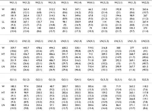
our consideration have exactly two parameters, we will use the negative of the log-likelihood as a measure of goodness-of-fit. This measure would result in the same conclusion as the Akaike's Information Criterion (AIC) [26]. Thus the smallest value suggests a better fit. We con-duct 1000 simulations with sample size of 200 and ran-dom censoring of approximately 40%. We sample time-to-event from 11 different parameter combinations of two parameter Weibull, log-normal and gamma distributions for a total of 33 combinations or 33000 simulations. We fit four mentioned models and average the -log likelihood over 1000 runs to determine which model fits the simu-lated data with the overall most precision on the average. Simulation results are presented in Table 1.
In simulations where we sample from a two-parameter Weibull distribution, obviously, the Weibull model fits the data with highest precision in all instances. Hyperta-bastic model is a close second, outperforming log-normal and log-logistic models for all combinations of parame-ters, with log-normal being the worst. Similarly when sampling is from a two-parameter log-normal distribu-tion, the log-normal model outperforms all other models. The hypertabastic model and the log-logistic show similar results, with the log-logistic being slightly better in eight combinations of parameters and the Weibull model per-forming the worst. Finally, when sampling from a two parameter gamma distribution, the Weibull model fits with the most precision in seven out of eleven combina-tions. That is because the Weibull distribution and the gamma distribution have hazard functions which are sim-ilar in shapes. In another four instances, the hypertabastic model slightly outperforms the Weibull model. The log-logistic model comes in third, however it is close to the hypertabastic and the Weibull for several combinations, while the log-normal does the worst in all instances.
8. Application
All models presented in the next two examples were fitted using Mathematica 6.0 (Wolfram Research, Inc.) and SASv9 (SAS Institute Inc., Cary, NC). They were fitted using both time and log(time). However, only log(time) results are presented for the multiple myeloma propor-tional hazards and brain cancer accelerated failure time models since log(time) is commonly used as a default approach in many packages and procedures. Besides the hypertabastic survival model we fit Weibull, log-normal, log-logistic and Cox models. We present all parameter estimates along with their standard errors and compare -2log-likelihood estimates, as well as AIC, to assess the goodness-of-fit of the models. SAS programs used to fit the hypertabastic proportional hazards models with time and log(time) for multiple myeloma data are provided [see Additional file 1].
LL(θ α β, , :X)= (lnSech α(−(Z t( )i)βCoth(Z t( )i )β )/β
1 + ( ( )) ( ) ( ) = − + ∑ i n i i i Z t
Csch Z t
1 1 2 2 δ α β β ln −− ( ( )) ( ( )) −( ( )) − +
α Z ti βCoth Z ti β Tanh α Z ti βCoth Z t
1
1
( ( ( )ii ) g Xi
( ) β )/β θ (8)
ALTLL(θ α β, , :X)= (lnSechα(−(Z t( )i)βCoth(Z t( )i)β)/β
1 + ( ( )) ( ) ( ) = − + ∑ i n
i i i
i
t Z t
Csch Z t
1 1 2 δ α β β ln − ( ( )) ( ( )) −( ( )) − + 2 1 1
αZ ti βCoth Z ti β Tanhα( Z ti βCooth(Z t( )i ) g Xi
8.1 Analysis of multiple myeloma data
Multiple myeloma is a cancer formed by abnormal white blood cells, called malignant plasma cells. A malignant monoclonal plasma cell is called plasmacytoma. If the disease spreads throughout multiple bone marrow sites in the body, it is called multiple myeloma. This disease weakens a patient's immune system and is usually diffi-cult to cure. To investigate the performance of the hyper-tabastic proportional hazards model and to compare it with Cox, Weibull, log-logistic and log-normal models, we analyze a cancer data set obtained from a study con-ducted by Krall et al. [27]. The data contains information on 65 patients with multiple myeloma in which the patients were treated with alkylating agents. This drug is designed to interfere with the cell's DNA and inhibits can-cer cell growth. Of these 65 patients, only 17 survived the duration of the study. The data is right-censored and the survival time from the date of diagnosis is measured in months. The covariates have been measured at diagnosis and the covariate list consists of a logarithm of white
blood cell count, serum calcium, presence or absence of Bence Jones protein, proteinuria, gender, age, percent myeloid cells in peripheral blood, percent lymphocytes in peripheral blood, logarithm of percent plasma cells in bone marrow, total serum protein, presence or absence of infection, serum globin, logarithm of blood urea nitro-gen, fractures, platelets, and hemoglobin. Our first task is to select risk factors that are statistically significant. To accomplish this task we use the hypertabastic log-likeli-hood function for proportional hazards model and follow the general variable selection strategy outlined by Collet [4]. We also examine the possibility of interactions. The two most significant risk factors that we found are the log-arithm of blood urea nitrogen and hemoglobin. Using the stepwise regression, we fit the Cox proportional hazards model. The Kaplan-Meier survival curve for multiple mye-loma data is shown in figure 2. The Cox regression did identify the same variables as the most significant prog-nostic factors. Table 2 gives results for the hypertabastic and the four comparison models. It shows that the
-2log-Table 1: Average -log likelihoods and their standard errors for Weibull (W), hypertabastic (HT), log-logistic (LL) and log-normal (LN) models based on 1000 simulations from eleven parameter combinations of two parameter Weibull, log-normal and gamma
distributions
W(1,1) W(1,2) W(2,1) W(1,3) W(3,1) W(1,4) W(4,1) W(.5,.5) W(.5,1) W(1,.5) W(2,3)
W 180.2 263.4 132 312.2 94.5 347.1 66.2 110.3 192.8 97.5 263.6 (8.8) (12.1) (6.8) (14.1) (8.6) (16.2) (9.2) (21.4) (21) (8.6) (10.7) HT 181.9 265.4 133.7 314.5 96.1 349.6 67.8 112.2 194.6 98.9 267
(9.1) (12.4) (7.1) (14.5) (8.9) (16.6) (9.3) (21.3) (21.1) (8.6) (11.2) LL 183.8 267.1 135.7 316 98.1 350.9 69.8 114 196.1 101.1 267.4 (9.3) (12.7) (7.3) (14.8) (9) (16.9) (9.3) (21.5) (21.3) (8.8) (11.4) LN 188.3 271.6 140 320.4 102.5 355.3 74 118.4 200.8 105.3 272
(10.4) (13.4) (8.6) (15.7) (8.1) (17.3) (10.3) (21.5) (21.7) (9.7) (11.4)
LN(1,1) LN(1,2) LN(2,1) LN(1,3) LN(3,1) LN(1,4) LN(4,1) LN(.5,.5) LN(.5,1) LN(1,.5) LN(2,3)
W 359.7 443.7 478.6 494.2 600.2 530.1 719.5 216.8 300 277 610.3 (18.6) (27) (23.6) (37) (30.4) (90.8) (34.7) (11.2) (15.5) (12.4) (41) HT 352.2 436.7 470.4 486.6 591.7 517.4 712 209.3 292.9 268.7 603.2
(17.6) (26.5) (23.1) (35) (29.7) (46.4) (34.1) (10.3) (14.9) (11.7) (40.6) LL 351.9 436.1 470.8 486.7 592.4 516.5 711.8 209 292.3 269.1 602.6 (17.6) (26.6) (23.1) (36.9) (29.7) (46.6) (34.2) (10.2) (15) (11.7) (40.7) LN 350.4 434.3 469.4 485.2 590.9 515 710.4 207.6 290.9 267.7 601.5 (17.6) (26.6) (23.1) (36.9) (29.6) (46.6) (34.2) (10.1) (14.9) (11.6) (40.5)
G(1,1) G(1,2) G(2,1) G(1,3) G(3,1) G(4,1) G(4,1) G(.5,.5) G(.5,1) G(1,.5) G(2,3)
Kaplan-Meier survival curve for multiple myeloma
Figure 2
Kaplan-Meier survival curve for multiple myeloma.
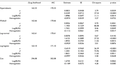
Table 2: Statistical results for hypertabastic proportional hazards and four comparison models for multiple myeloma data
-2Log likelihood AIC Estimate SE Chi-square p-value
Hypertabastic 162.33 170.33
α 0.0853 0.0438 3.79 0.0559
β 0.4349 0.0712 37.34 <0.0001 Log(BUN) 1.8986 0.5697 11.11 0.0014 Hemogolobin -0.0974 0.0539 3.27 0.0752 Weibull 162.66 170.66
α 0.0056 0.0067 0.70 0.4041
β 1.1403 0.1229 86.08 <0.0001 Log(BUN) 1.7451 0.5999 8.46 0.0049 Hemogolobin -0.1112 0.0561 3.93 0.0517 Log-normal 162.61 170.61
α 0.0078 0.0095 0.67 0.4145
β 1.6153 0.3089 27.35 <0.0001 Log(BUN) 1.8935 0.5703 11.02 0.0015 Hemogolobin -0.0929 0.0536 3.01 0.0876 Log-logistic 163.10 171.10
α -5.6519 0.9369 36.39 <0.0001
β 1.2401 0.1452 72.96 <0.0001 Log(BUN) 1.8651 0.5464 11.65 0.0011 Hemogolobin -0.0997 0.0526 3.58 0.0628 Cox 296.08 302.08
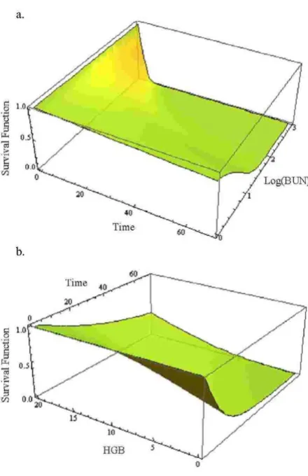
likelihood and AIC statistics are lowest for the hypertabas-tic model when fitted to the multiple myeloma data. This indicates that the hypertabastic proportional hazards model fits the multiple myeloma data best. The most sig-nificant single variable identified by the hypertabastic model is the logarithm of blood urea nitrogen with an estimated chi-square value of 11.11 (p = 0.0014). The sec-ond significant variable is hemoglobin. All other models have identified these two variables as the most significant ones. The mean levels of patients' hemoglobin and the logarithm of blood urea nitrogen are 10.20 and 1.39 respectively. At this level, the median survival time for the hypertabastic, log-normal, log-logistic, Weibull and Cox are 20.04, 19.29, 21.01, 21.92 and 19 months respec-tively. Figures 3a and 3b show the graph of hypertabastic hazard and survival functions for multiple myeloma data. Figure 3a clearly shows that the hypertabastic hazard func-tion is an increasing funcfunc-tion of time. By examining figure 3b, we realize that for patients with a Log (BUN) reading of 1.39 and a hemoglobin level of 10.20 there is about a10% chance of survival beyond 65 months. At the above mentioned mean levels for the hemoglobin and loga-rithm of blood urea nitrogen, the hypertabastic hazard function shows that the failure rate (hazard) reaches its maximum velocity in about 5.15 months. At this point the disease progression has its highest speed (Figure 3c). Figures 4a and 4b show the 3-dimensional graphs for sur-vival of multiple myeloma patients as functions of time and Log(BUN), as well as time and HGB. Other models under consideration had monotone increasing hazard functions (graphs not shown).
8.2 Analysis of glioma brain cancer data
Glioma is a cancer of the brain which begins in glial cells. These cells support the neurons. These cells have a very high rate of growth which can quickly destroy the normal cells. The primary types of glioma cancers are astrocyto-mas, ependymomas and oligodendrogliomas. Shin et al. [28] studied ways to improve the effectiveness of radia-tion in the treatment of cerebral malignant astrocytoma. Their study focused on the assessment of the effect of mul-tiple daily fractionated radiation therapy with and with-out misonidazole. They concluded that the addition of misonidazole did not significantly improve the patients' survival. In this section we apply the hypertabastic accel-erated failure time technique to model the survival time of a sample of 30 patients from the randomized trials of radi-otherapy with and without the radiosensitizer misinida-zole. The data was obtained from the Medical Research Council Working Party (MRC) on misonidazole in glio-mas. This data is right censored and has been previously analyzed for the selection of variables by MRC [29]. Sur-vival time was measured in days and the longest surSur-vival time was 1098 days. We compared radiotherapy treat-ment of brain cancer patients with radiosensitizer
misoni-dazole to radiotherapy without misonimisoni-dazole. Figure 5 shows a Kaplan-Meier plot of the estimated survival curves for both groups. The log-rank, Wilcoxon, and like-lihood ratio tests are all non-significant, suggesting no sig-nificant difference between survival curves for the two groups. The Kaplan-Meier estimates of median survival time for radiotherapy with misonidazole group is 258.5 days and for the radiotherapy without misonidazole group is 488 days. The overall median survival time for both groups combined is 361 days. Using the
Kaplan-a) Hypertabastic hazard curve for multiple myeloma; b) Hypertabastic survival curve for multiple myeloma; c) Hyper-tabastic velocity of hazard curve for multiple myeloma
Figure 3
Meier estimates of survival function, a plot of log-cumula-tive hazard function against the logarithm of the survival time for individuals in two groups indicates that the data is coming from a Weibul distribution. Knowing this infor-mation led us to evaluate the performance of the hyperta-bastic model. First, we fit a hypertahyperta-bastic accelerated failure time model to analyze the brain cancer data. Then the hypertabastic accelerated failure time model is com-pared with Weibul, log-logistic, log-normal accelerated failure time models and the Cox proportional hazards model. This model incorporates a binary covariate coded as treatment = 1 for the type of radiotherapy with misoni-dazole, and as treatment = 0 for radiotherapy without mis-onidazole. The second covariate is the age of the patient. Thus, this model contains two covariates- treatment and age. We use the method of maximum likelihood to maxi-mize hypertabastic accelerated failure time log-likelihood function for right censored data discussed in section 5.
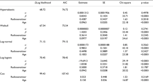
Table 3 gives a statistical summary for the glioma data. For instance, the hypertabastic estimated value for the coeffi-cient of the variable radiosensitizer is 0.4387 with a stand-ard error of 0.3437. The Wald and the likelihood ratio statistics associated with this variable are 1.6294 (p = 0.2018) and 1.6254 (p = 0.2023) respectively. Both tests indicate that the effect of individual variable radiosensi-tizer is non-significant. The estimated accelerator factor is 1.5507 (exponentiated value of parameter 0.4387). This means that after controlling for the age of the patient, the probability of a patient treated with "therapy with radio-sensitizer misonidazole" surviving t days equals to the probability of a patient treated with "therapy without radiosensitizer misonidazole" surviving 1.5507 t days. For instance, the hypertabastic accelerated failure time model suggests that for 49 year old patients (median age for all patients under study), the probability of a patient treated with " therapy with radiosensitizer misonidazole " surviv-ing 293 days equals to the probability of a patient treated with" therapy without radiosensitizer misonidazole " sur-viving 454 days. The Wald statistic for the age covariate is 22.18 (p < 0.0001).
Using AIC, we came to the conclusion that both Weibull and hypertabastic models fit the data very well. However, the Weibull AIC value was 75.54 which indicates the best fit. For the hypertabastic model, the AIC value was 76.72 which was slightly less than Weibull. The remaining AIC values for log-normal, log-logistic and Cox are 79.15, 78.45, and 107.43 respectively. At the median age of 49, the median survival time for those patients who under-went radiotherapy with radiosensitizer misonidazole using the hypertabastic, Weibul, log-normal, log-logistic, and the Cox models are 289, 316, 270, 277, and 244 days respectively. The corresponding median survival times for the group without the radiosensitizer misonidazole are 449, 453, 423, 456, and 488 days respectively. By examin-ing the Kaplan-Meier survival functions for the two groups we observe the crossing pattern which is a clear indication of violation of proportional hazards assumption. Figures 6a and 6b show the graphs of hypertabastic hazard and survival functions for both treatment groups at the age level of 49. The hazards for both groups are increasing function of time. For those patients who received radio-therapy treatment with radiosensitizer misonidazole, haz-ard function reached its maximum velocity in about 200 days. For those who did receive radiotherapy without mis-onidazole, hazard function reached its maximum velocity in about 311 days. These are the points in time where the speeds of failure rates (hazards) are highest (Figure 6c). Figures 7a and 7b represent 3-dimensional graphs of sur-vival by time and age for each treatment group separately.
a) Hypertabastic 3D survival curve with variables time and Log (BUN) for multiple myeloma data; b) Hypertabastic 3D survival curve with variables time and HGB for multiple mye-loma data
Figure 4
Kaplan-Meier survival curves for glioma brain cancer
Figure 5
Kaplan-Meier survival curves for glioma brain cancer.
Sur
vi
val Distri
bution
Function
Days
Without Misonidazole With Misonidazole
Table 3: Statistical results for the hypertabastic accelerated failure time model and four comparison models for glioma brain cancer data
-2Log likelihood AIC Estimate SE Chi-square p-value
Hypertabastic 68.72 76.72
α 0.0001312 0.0001956 0.45 0.4978
β 0.8343 0.1434 33.71 <0.0001 Radiosensitiser 0.4387 0.3437 1.63 0.2018
Age 0.0963 0.0205 22.18 <0.0001 Weibull 67.54 75.54
α 0.0000003 0.0000007 0.12 0.2741
β 1.4203 0.2456 33.44 <0.0001 Radiosensitiser 0.3614 0.3040 1.41 0.2345
Age 0.0977 0.0197 24.61 <0.0001 Log-normal 71.15 79.15
α 0.0000173 0.0000188 0.85 0.3563
β 0.9853 0.1501 43.10 <0.0001 Radiosensitiser 0.4498 0.3889 1.37 0.2427
Age 0.1003 0.0207 23.58 <0.0001 Log-logistic 70.45 78.45
α -19.6913 3.6445 29.19 <0.0001
β 1.8338 0.3251 31.82 <0.0001 Radiosensitiser 0.5000 0.3718 1.81 0.1787
Age 0.0942 0.0208 20.52 <0.0001 Cox 99.43 107.43
9. Discussion and conclusion
In this paper we have introduced a new survival model called hypertabastic survival model. The overall results of our simulation indicate that the hypertabastic model per-forms best when the data is generated from the Weibull distribution. When the data comes from the gamma dis-tribution, both the Weibull and hypertabastic distribu-tions perform well. In the case when we generate survival data from the log-normal distribution, the log-logistic and
hypertabastic distributions perform well but the gamma and Weibull perform poorly. In the last case, the Weibull distribution performance is the worst. We believe that the hypertabastic survival model is to some extent robust with respect to variations in the distribution. We believe that the hypertabastic hazard function can play a role in mod-eling failure rates in medical, biological and engineering fields. The hypertabastic model can also assist physicians and clinicians with their treatment planning through its ability to predict patients' outcome as well as the risk of disease recurrence. Gilbert et al. [30] argued that the pat-tern of instantaneous risk over time is more interesting than the cumulative risk. For instance, in a cancer study where recurrence time of malignant tumor is of interest, a bimodal hazard curve may represent the elevated
inci-a) Hypertabastic 3D survival curve with variables time and age for group using radiotherapy with radiosentisizer misoni-dazole for glioma brain cancer; b) Hypertabastic 3D survival curve with variables time and age for group using radiother-apy without radiosentisizer misonidazole for glioma brain cancer
Figure 7
a) Hypertabastic 3D survival curve with variables time and age for group using radiotherapy with radiosentisizer misoni-dazole for glioma brain cancer; b) Hypertabastic 3D survival curve with variables time and age for group using radiother-apy without radiosentisizer misonidazole for glioma brain cancer.
a) Hypertabastic hazard curves for glioma brain cancer; b) Hypertabastic survival curves for glioma brain cancer; c) Hypertabastic velocity of hazard curves for glioma brain can-cer
Figure 6
dences of early and late recurrences and the magnitude of the hazard rates at the peaks may reveal the intensity of the failure rates. Therefore we recommend that clinicians, practitioners and analysts consider using this model along with other models, and compare it to the models they ordinarily use before making any decision as to which model would provide the best fit and prediction.
Competing interests
The author(s) declare that they have no competing inter-ests.
Authors' contributions
The survival model equations were developed by MAT and ZB based on their previous work on hyperbolastic growth and survival models. Applications of the models to data were done by MAT, ZB, DKW and KPS. Writing of the manuscript was done by MAT and ZB, and final edits by DKW and KPS.
Additional material
References
1. Hosmer DW, Lemeshow S: Applied Survival Analysis:
Regres-sion Modeling of Time to Event Data. New York: Wiley; 1999.
2. Lee ET, Wang JW: Statistical Methods for Survival Data Analysis 3rd
edi-tion. New York: Wiley; 2003.
3. Kleinbaum DG, Klein M: Survival Analysis: A Self-learning Text 2nd
edi-tion. New York: Springer; 2005.
4. Collet D: Modeling Survival Data in Medical Research New York:
Chap-man and Hall/CRC; 1994.
5. Cox DR: Regression Models and Life Tables. Journal of the Royal
Statistical Society, Ser B 1972, 34:187-220.
6. Efron B: The Efficiency of Cox's Likelihood Function for
Cen-sored Data. Journal of the American statistical Association 1977,
72:557-656.
7. Lee ET, Go OT: Survival Analysis in Public Health Research.
Annual Reviews in Public Health 1997, 18:105-134.
8. Simes RJ, Zelen M: Exploratory Data Analysis and the Use of
the Hazard Function for Interpreting Survival Data: An Investigator's Primer. Journal of Clinical Oncology 1985, 3:418-431.
9. Tabatabai M, Williams DK, Bursac Z: Hyperbolastic Growth
Mod-els: Theory and Application. Theoretical Biology and Medical Mod-eling 2005, 2:1-13.
10. Bursac Z, Tabatabai M, Williams DK: Non-linear Hyperbolastic
Growth Models and Applications in Cranofacial and Stem Cell Growth. In 2005 Proceedings of the American Statistical Associa-tion Biometrics SecAssocia-tion [CD-ROM], Alexandria, VA: American Statis-tical Association; 2006:190-197.
11. Goodman MS, Li Y, Tiwari RC: Survival Analysis with Change
Point Hazard Functions. Harvard University Biostatistics Working Paper Series 2006. Working Paper 40
12. Lundin J, Lundin M, Isola J, Joensuu H: Evaluation of a Web-based
System for Survival Estimation in Breast cancer. Studies in Health Technology and Informatics 2003, 95:788-793.
13. Royston P, Parmar MK: Flexible Parametric
Proportional-haz-ards and Proportional-odds Models for Censored Survival Data, with Application to Prognostic Modeling and Estima-tion of Treatment Effects. Statistics in Medicine 2002,
21:2175-2197.
14. Kay R, Schuerlen H, Schumacher M: On the Use of Hazard
Func-tions in Breast Cancer Studies. Experientia Supplement 1982,
41:118-130.
15. Foulkes MA, Sacco RL, Mohr JP, Hier DB, Price TR, Wolf PA:
Para-metric Modeling of Stroke Recurrence. Neuroepidemiology 1994, 13:19-27.
16. Sama W, Dietz K, Smith T: Distribution of Survival Times of
Deliberate Plasmodium Falciparum Infections in Tertiary Syphilis Patients. Transactions of the Royal Society of Tropical Medi-cine and Hygiene 2006, 100:811-816.
17. Kannan N, Raychaudhuri A, Pilamanis AA: A Log logistic Model for
Altitude Decomposition Sickness. Aviation, Space and Environ-mental Medicine 1998, 69:965-970.
18. Nardi A, Schemper M: New Residuals for Cox Regression and
Their Application to Outlier Screening. Biometrics 1999,
55:523-529.
19. Nardi A, Schemper M: Comparing Cox and Parametric Models
in Clinical Studies. Statistics in Medicine 2003, 22:3597-3610.
20. Chen YQ: Accelerated Hazards Regression Model and its
Adequacy for Censored Survival Data. Biometrics 2001,
57:853-860.
21. Clark TG, Stewart ME, Altman DG, Gabra H, Smyth JF: a Prognostic
Model for Ovarian Cancer. British Journal of Cancer 2001,
85:944-952.
22. Demicheli RM, Bonadonna G, Hrushesky WJ, Retsky MW, Valagussa
P: Menopausal Status Dependence of the Timing of Breast Cancer Recurrence After Surgical Removal of the Primary Tumor. Breast Cancer Research 2004, 6:689-696.
23. Schulman LL, Weinberg AD, McGregor CC, Suciu-Foca NM, Itescu S:
Influence of Donor and Recipient HLA Locus Mismatching on Development of Obliterative Bronchiolitis after Lung Transplantation. American Journal of Respiratory and Critical Care Medicine 2001, 163:437-442.
24. Weitz JS, Fraser HB: Explaining mortality rate plateaus.
Proceed-ings of the National Academy of Science 2001, 98:15383-15386.
25. Chan PL, Holford NH: Drug Treatment Effects on Disease
Pro-gression. Annual Reviews of Pharmacology and Toxicology," 2001,
41:625-659.
26. Akaike A: A New Look at the Statistical Model Identification.
IEEE Trans Autom Control AC 1974, 19:716-723.
27. Krall JM, Utoff VA, Harley JB: A Step-up Procedure for Selecting
Variables Associated with Survival. Biometrics 1975, 31:49-57.
28. Shin KH, Urtasun RC, Fulton D, Geggie PHS, Tanasichuk H, Thomas
H, Muller PJ, Curry B, Mielke B: Multiple Daily Fractionated
Radi-ation Therapy and Misonidazole in the Management of Malignant Astrocytoma. Cancer 1985, 56:758-760.
29. Medical Research Council Working Party: A study of the effect of
misonidazole in conjunction with radiotherapy for the treat-ment of grades 3 and 4 astrocytomas. A report from the MRC Working Party on misonidazole in gliomas. Br J Radiology 1983, 56:673-682.
30. Gilbert PB, Wei LJ, Kosorok MR, Clomens JO: Simultaneous
Infer-ences on the Contrast of Two Hazard Functions with Cen-sored Observations. Biometrics 2002, 58(4):773-780.
Additional file 1
Hypertabastic model fitting to multiple myeloma data using SAS PROC NLP. SAS PROC NLP code provided here demonstrates how to fit hyper-tabastic model to multiple myeloma data using both time and log(time). Click here for file