Article
Quantifying bioirrigation using ecological parameters:
a stochastic approach
{
Carla M. Koretsky,*
aChristof Meile
band Philippe Van Cappellen
ba
Department of Geosciences, Western Michigan University, Kalamazoo, MI, USA. Tel: 616 387 5337; Fax: 616 387 5513; E-mail: [email protected]
b
Faculty of Earth Sciences, Utrecht University, 3508 TA Utrecht, . E-mail: [email protected]; [email protected]; Fax: 31 30 253 5302; Tel: 31 30 253 5005
Received 15th November 2001, Accepted 5th February 2002
Published on the Web 20th February 2002First published as an Advanced Article on the web 19th October 2001
Irrigation by benthic macrofauna has a major influence on the biogeochemistry and microbial community structure of sediments. Existing quantitative models of bioirrigation rely primarily on chemical, rather than ecological, information and the depth-dependence of bioirrigation intensity is either imposed or constrained through a data fitting procedure. In this study, stochastic simulations of 3D burrow networks are used to calculate mean densities, volumes and wall surface areas of burrows, as well as their variabilities, as a function of sediment depth. Burrow networks of the following model organisms are considered: the polychaete worms Nereis diversicolorandSchizocardium sp., the shrimpCallianassa subterranea, the echiuran wormMaxmuelleria lankesteri, the fiddler crabsUca minax,U. pugnaxandU. pugilator, and the mud crabsSesarma reticulatum andEurytium limosum. Consortia of these model organisms are then used to predict burrow networks in a shallow water carbonate sediment at Dry Tortugas, FL, and in two intertidal saltmarsh sites at Sapelo Island, GA. Solute-specific nonlocal bioirrigation coefficients are calculated from the depth-dependent burrow surface areas and the radial diffusive length scale around the burrows. Bioirrigation coefficients for sulfate obtained from network simulations, with the diffusive length scales constrained by sulfate reduction rate profiles, agree with independent estimates of bioirrigation coefficients based on pore water chemistry. Bioirrigation coefficients for O2derived from the stochastic model, with the diffusion length scales constrained by O2microprofiles
measured at the sediment/water interface, are larger than irrigation coefficients based on vertical pore water chemical profiles. This reflects, in part, the rapid attenuation with depth of the O2concentration within the
burrows, which reduces the driving force for chemical transfer across the burrow walls. Correction for the depletion of O2in the burrows results in closer agreement between stochastically-derived and
chemically-derived irrigation coefficient profiles.
Introduction
Nearshore sediments support large populations of burrowing macroinfauna, such as polychaete worms, shrimps and crabs. These organisms build extensive burrow networks within the upper 10 to 100 cm of the sediment column, which are either passively or actively flushed with water from the overlying sediment/water interface (SWI). Differences in solute concen-trations between water flushed through burrows and pore water in the surrounding bulk sediment provide the driving force for enhanced solute mass transfer, called bioirrigation.1–3 Bioirrigation not only enhances solute fluxes,4,5 but also influences the microbial community structure,6–9 as well as sediment and pore water composition.10–15
Mathematical one-dimensional (1D) models of bioirrigation have been developed that treat bioirrigation variously as a diffusive, advective or nonlocal process. Diffusive models of bioirrigation use increased diffusion coefficients to account for enhanced solute transport due to macrofaunal activity within a defined mixing zone.16–20 A diffusive representation implies
that biological solute mixing is rapid and occurs on a spatial
scale much smaller than the characteristic length scale of chemical pore water gradients.21Less common are advective models of bioirrigation, in which an enhanced advection velocity accounts for increased vertical pore water trans-port.11,22,23 Boudreau24 and Boudreau and Imboden25 have argued that a more appropriate description of bioirrigation is based on a nonlocal transport description. The most common approach employs a mass transfer coefficient or bioirrigation coefficient, a, to describe the rate of exchange between overlying water and pore waters at depth.12,26,27None of the
1D bioirrigation models, however, include an explicit repre-sentation of the burrow networks constructed by the resident macrofaunal populations.
An important step in bridging the gap between chemical transport modeling of bioirrigation and benthic ecology was the development of the 3-dimensional (3D) radial diffusion model by Aller.1In this approach, burrows are represented as
continuously flushed, evenly spaced cylindrical burrows of constant diameter and depth. Solutes are transported diffu-sively across the burrow walls in response to concentration gradients between bulk pore waters and waters flushed into burrows from the overlying SWI. Boudreau and Marinelli extended the 3D burrow model to describe discontinuous flushing of burrows, as well as variations in animal population (distance between burrows) and organism sizes (burrow radii).5 Boudreau further showed that the 1D nonlocal description of {Presented during the ACS Division of Geochemistry symposium
‘Biogeochemical Consequences of Dynamic Interactions Between Benthic Fauna, Microbes and Aquatic Sediments’, San Diego, April 2001.
irrigation is equivalent to the 3D model of continuously flushed vertical cylinders; the 1D nonlocal equation is simply the radially integrated form of the 3D model.28The equivalence between the 3D burrow model and the 1D nonlocal model implies that the magnitude of bioirrigation at a given depth depends critically on the burrow wall surface area at that depth. In all of the above models (diffusive, advective, nonlocal and cylindrical burrow) assumptions are made regarding the depth dependence of the intensity of bioirrigation. Bioirrigation intensity is either assumed to be constant over a discrete interval, or a functional depth-dependence is assigned to enhanced diffusion coefficients or nonlocal exchange coeffi-cients.12,13,29,30 Values of irrigation coefficients are generally derived by fitting chemical profiles, rather than by relying on ecological information. However, in principle, the latter could be used to determine the depth dependence of bioirrigation intensity directly. In addition, the models discussed so far are strictly deterministic and provide no information concerning the spatial or temporal variability of irrigation.
In this study, a stochastic model of bioirrigation based on benthic ecological data is presented. Information on burrow sizes and shapes for a variety of representative macrofaunal organisms is used to calculate stochastic realizations of 3D burrow networks. By generating a large number of burrow networks it then becomes possible to determine both average burrow surface areas and their variability as a function of depth. Benthic ecologists have characterized the structures of burrows using methods such as resin casting and X-radio-graphy; these detailed measurements can be used to calculate the depth-dependence of burrow surface areas without implementing a stochastic approach. However, the stochastic model presented here is advantageous because it can also be used to provide estimates of surface area variability. Surface areas from the stochastic model provide an independent method for constraining the depth dependence of irrigation coefficients used in 1D nonlocal models of bioirrigation. The stochastic model also provides a method to assess the uncertainty associated with irrigation coefficients in sediments.
Model
The stochastic burrow network
In the stochastic model, the sediment is represented as a 3D grid over which burrows are distributed. Burrows are modeled using ten endmember shapes commonly observed in macrofaunal burrow networks (Fig. 1). The following input parameters, with corresponding standard deviations and probability distributions where appropriate, are user-specified: (1) total burrow density (burrows per m2), (2) probability of
occurrence for each of the 10 possible burrow shapes, and (3) radius and lengths of segments associated with each burrow shape. For example,U-shaped burrows require specifications for vertical and horizontal segment lengths;Y-shaped burrows require specifications for lengths of inclined upper branches and for the horizontal stem.
With the specified input parameters, burrows are distributed
over the grid as follows. For each realization of the network a total burrow density is chosen randomly from the user-specified probability distribution of the total burrow density. The total burrow density is partitioned among the different burrow shapes based on the user-specified probabilities of occurrence of the ten possible burrow shapes. For each burrow, the lengths of the burrow segments and the radius of the burrow are selected similarly using the corresponding prob-ability distributions. For nonvertical burrow orientations, the direction of the horizontal or inclined burrow section is selected randomly as north, south, east or west, with equal probability for each direction.
After all of the burrow parameters have been calculated, the burrow is placed into the 3D network of grid blocks. Each block either contains bulk sediment or is part of a burrow. The location of the burrow is determined by generating random coordinates for the burrow exit at the top surface of the grid (i.e., at the SWI). For each burrow type, the user specifies whether the burrow is allowed to intersect with other burrows. If the calculated exit coordinates cause the burrow to intersect with another burrow, and no intersection is allowed, the exit coordinates are recalculated until the burrow can be located in the grid, or until a large number of attempts (specified by the user) is exceeded, ending the simulation. To eliminate edge effects, burrows that exit the grid sides are continued at the opposite edge (i.e., a periodic boundary condition is imposed). For all stochastically generated parameters, either a Rayleigh or Gaussian probability distribution function may be selected, or the parameter may be specified deterministically for use in all simulations.
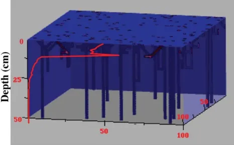
For each stochastic realization of the burrow network (Fig. 2), the burrow volume, density and burrow wall surface area are calculated within each depth interval of the 3D grid. To calculate surface areas, all burrows are treated as cylindrical tubes. The surface area (sh) per unit sediment depth of vertical
or horizontal burrows is therefore equal to
sh~
b<450:2pr1 cosb
b§450:2pr1 sinb (
(1)
wherer1is the burrow radius,bis the angle of the burrow with
respect to the vertical, and the subscript h indicates that the surface area within the depth interval is normalized to the uniform grid spacing, h. The total burrow surface area per unit sediment depth,Sh, at any given depth is then obtained by:
Sh~
X
sh (2)
where summation is carried out over all the burrows in the given depth interval. For simplicity, in the case of intersecting burrows, the surface area at the grid point of intersection is that calculated for the last burrow placed in the grid block. Because
Fig. 1 Endmember shapes used in stochastic burrow network simulation.
burrows are placed into the grid randomly and many networks are simulated, this results in an averaging of intersecting large and small surface area burrows. The mean values and standard deviations of the burrow density and burrow surface area are calculated as a function of depth by performing a large number of successive burrow network simulations (default 10 000 simulations).
Burrow networks and nonlocal exchange coefficients
Derivation of nonlocal exchange coefficients from burrow surface areas. Bioirrigation occurs because burrows provide conduits for solute mass transport that is rapid relative to diffusion through the bulk sediment. The burrow network therefore significantly influences biogeochemical cycling in the sediment. This is especially true in nearshore environments, where biologically mediated transport is often the dominant solute transport mechanism in surface sediments.31Studies that attempt to link observed pore water profiles with the under-lying process dynamics thus require a mathematical description of solute exchange due to bioirrigation. One such model is the nonlocal exchange coefficient description of bioirrigation,26 where the rate at which a solute is added or removed by bioirrigation (Inl) at a given depth in the sediment is given by
Inl(x)~aiw(C0{Cavg)
x, (3)
where w is the sediment porosity, and the bioirrigation co-efficient, ai, in units of inverse time, denotes the nonlocal
exchange coefficient describing mass transfer of a given solute, i, between the overlying water and the bulk sediment;C0and
Cavgare the solute concentrations in the overlying water and in
the bulk sediment, respectively.
Boudreau has demonstrated that the nonlocal exchange coefficient description of bioirrigation is equivalent to the continuously flushed radial tube model of bioirrigation developed by Aller.1,28He proposes the following equation:
Inl~{ 2Diw
r2 2{r21
r1 LC Lr r1 , (4)
whereDiis the molecular diffusion coefficient of thei-th species
corrected for tortuosity,r1the radius of the vertical, cylindrical
burrows,r2the half-distance between burrows, and (hC/hr) the
concentration gradient of soluteiextending from the burrow wall into the bulk sediment. In the idealized radial tube model, the term 2r1/(r222r12) corresponds to the burrow surface area
per volume of sediment surrounding an individual burrow (sv).
The main difficulty in applying eqn. (4) resides in estimating (hC/hr). If we approximate the concentration gradient by a truncated Taylor series expansion, then
LC Lr r 1
&Cavg{Cb
ri{r1
(5)
wherer¯iis the (time averaged) distance from the burrow wall at
which the solute concentration reaches the radially averaged concentration,Cavg, for the bulk sediment at a given depth and
Cbis the (time averaged) concentration in the burrow.
If the total burrow volume is relatively small (i.e.,r1%r2),
the volume of bulk sediment surrounding an individual burrow at a given depth is approximately equal to the total sediment volume divided by the number of burrows at that depth. Therefore, sv # Sv, where Sv is the burrow surface area
summed over all burrows divided by the total volume of sediment modeled within a given depth interval. At the sites assessed in this study (Dry Tortugas, FL and Sapelo Island, GA), the contribution of burrows to total sediment porosity is small (v5%), justifying this simplification. If we assume that the solute concentrations within burrows are similar to the
concentrations in the overlying water (Cb# C0) then, using
eqn. (3)–(5), it follows that
ai,0~{
2Dir1 (r2
2{r21)(C0{Cavg) LC Lr r1
&{ DiSv
(C0{Cavg) LC Lr r1
&Di
Sv
ri{r1
(6)
Eqn. (6) is derived for the idealized model of evenly spaced, identical vertical burrows. In this study, we assume that, within each horizontal slice of the 3D sediment grid, eqn. (6) provides a good approximation for the relationship between the bio-irrigation intensity and the size and density of burrows. The stochastic burrow network can then be used to calculate mean values of burrow surface areas and radii, which can be implemented in eqn. (6). While the assumption underlying the equivalence between 1D nonlocal irrigation coefficients and idealized 3D cylindrical burrows is not strictly met for complex burrow geometries, the approach provides a means to estimate the depth-dependence of a, which is otherwise poorly constrained.
The equivalent burrow radius r1(x) is calculated from the
total burrow surface area per unit sediment depth according to
r1(x): Sh(x) 2pntot(x)
, (7)
wherentot(x) is the total number of burrows encountered in the
depth interval over whichShis determined. BothntotandShare
calculated from the stochastic realizations of the 3D burrow network. Eqn. (7) accounts for the fact that inclination of the burrows with respect to the vertical increases the surface area available for exchange between burrows and bulk sedi-ment.31,32The average half-distance between burrows may be required for estimation of r¯i (see below). It is obtained by
analogy with an ideal closest packing arrangement of vertical burrows,i.e.burrows (and the cylindrical packet of sediment surrounding each burrow) are assumed to be distributed evenly over the grid. The average half-distance between burrows at a given depthx, is then given by
r2(x)~
ffiffiffiffiffiffiffiffiffiffiffiffiffiffiffiffiffiffiffiffiffiffiffi
1 2pffiffiffi3
A0 ntot(x)
s
(8)
wherentot(x) is the mean total number of burrows encountered
in the sediment slab, andA0is the horizontal surface area of the
3D grid.
Diffusion length scales. From eqn. (6) it is evident that the irrigation coefficient may depend on the chemical species, not only through the species-specific diffusion coefficient, but also through a characteristic radial diffusion length scale, Li ~
r¯i2r1. In theory, the latter can be obtained by direct
measure-ments of chemical microprofiles across at the burrow/sediment interface (BSI). Such data, however, are rarely available. Alter-natively, vertical microprofiles recorded at the sediment/water interface (SWI) may be used as analogs for the gradients at the BSI, or the radial diffusion length scales may be estimated from simplified reaction-transport models.
If vertical diffusion at the SWI is considered analogous to radial diffusion at the BSI, the measured vertical length scale of the concentration change at the SWI (Li’) must be corrected to
unit area of surface extending to depth Li’, divided by the
surface area of the sediment isLi’. This must be equal to the
ratio of sediment volume associated with an individual burrow to the burrow’s surface area,
L’i~
Ðri
r1 2prdr
2pr1
(9)
which yields
ri~
ffiffiffiffiffiffiffiffiffiffiffiffiffiffiffiffiffiffiffiffiffiffiffiffiffiffiffiffiffiffiffi
r2
1(x)z2r1(x)L’i q
(10)
The radial diffusion length scale r¯ipredicted by eqn. (10) is
strictly speaking only valid near the SWI, where Li’ reflects
the local production or consumption of the solute. As the production (consumption) rate changes with depth, so will the value ofr¯i.
When measurements of rates of consumption or production of the solute in the bulk sediment are known, it is possible to estimate values ofLiby assuming that in close proximity of
burrows solute transport is dominated by irrigation (i.e., vertical diffusion can be ignored). From the vertical profiles of solute concentration and net rate of production/consumptiona can be determined by balancing the flux across the burrow walls with the reaction taking place in the surrounding sediment,
{Diw
LC Lr r 1 2pr1~
ð r2
r1
wRi2prdr (11)
Using the approximation of eqn. (5), and assumingCb#C0,
the corresponding length scale at the BSI forr2&r1is then
Li~2Di
r1(C0{Cavg) r2
2Ri
(12)
whereRiis the net rate of production/consumption in the bulk
sediment expressed per unit pore water volume.
Estimates of length scales and bioirrigation coefficients can also be obtained if the reaction kinetics are known and the governing mass balance equation is solved at steady state, with the average concentration defined as
Cavg~
ð r2 r1 rC(r)drz ð r1 0 rC0dr
0 @
1
A, ð
r2
0 rC0dr
0 @
1
A (13)
Subsequently,r¯ican be determined using the conditionC(r¯i)~
Cavg. For example, for zeroth order kinetics,
0~Di r L Lr r LC Lr
{Ri (14)
With the boundary conditionsC(r1)~C0and (hC/hr) atr2~
0, the radial concentration profile is given by
C(r)~C0{ Ri
4Di
(r2 1{r2){
Rir22 2Di
ln r r1
(15)
Solving forr¯ileads to
r~exp {f(x)
2 {
3
4zln(r2)z r2 1 2r2 2 { r 4 1 4r4 2 ,
x~{r{22exp(y),
y~({r{4
2 (1:5r42{2r42ln(r2){r22r21z0:5r41))
(16a)
wheref(x) fulfillsf(x)?ef(x)~x. For |x|v0.3,f(x), the Lambert W function, can be expressed with a relative errorv1% in a series expansion,
f(x)&x{x2z3x3 2 { 8x4 3 z 125x5 24 { 154x6 5 z16807x 7 720 { 16384x8 315 z 1531441x9 4480 (16b)
From eqn. (16) it is apparent that for zeroth order kinetics,r¯i
depends only on the burrow size and spacing, not on the reaction rate or diffusion coefficient. Thus, the expected species specificity ofaonly results from the species dependence of the effective diffusion coefficient. For other reaction kinetics,1,33 numerical methods are required to determiner¯i.
Burrow flushing efficiency. Nonlocal transport models of irrigation generally assume perfectly efficient flushing of burrows, that is Cb ~ C0 (eqn. (3), (6). If perfect flushing
does not occur, then depletion (or accumulation) of the solute within the burrow will cause the nonlocal irrigation coefficient, ai,b(x) to deviate from the apparent irrigation coefficient,ai,0(x)
defined by eqn. (3). The relationship between the true irrigation coefficient (ai,b) and the apparent coefficient is
ai,b&{ DiSv (C0{Cavg)
LC Lr r 1
&Di
Sv (C0{Cavg)
(Cb{Cavg) (ri{r1)
~ai,0
(Cb{Cavg) (C0{Cavg)
(17)
For highly reactive species, or small burrows, this effect may significantly affect bioirrigation coefficient profiles. From eqn. (17), it can be seen that the bioirrigation intensity is species-specific, becauseCbandC, and therefore the ratio of (Cb2C)/
(C02C), depend on the reactivity and diffusion coefficient of
the individual solute species.
To assess the significance of concentration changes in bur-rows, the steady state concentration profile within a burrow can be estimated. Balancing the net delivery of the solute to a given depth by flushing of a vertical burrow with radial exchange across the burrow wall gives
QLCb
Lx ~2pr1.Diw LC Lr r 1 (18)
whereQis the volumetric flux of water flushing through the burrow. Q is obtained either by direct measurement or is estimated iteratively using the depth-integrated irrigation coefficient profile. Advective water velocity in the burrow is related to the mass flux of water byu~Q/(pr12). If the average
concentration of the solute in the bulk sediment remains approximately constant (e.g., in the case of O2which is rapidly
depleted near the SWI, so thatCavg#0 over most of the depth
range of interest), then the radial derivative in eqn. (18) can be expressed according to eqn. (5), or
LCb Lx ~{
2Diw
r1uLi
(Cb{Cavg) (19)
Solving eqn. (19) for the boundary condition Cb(0) ~ C0
gives
Cb(x)~(C0{Cavg)e {2Diw
r1uLixzCavg (20)
which shows, as expected, that deviation from perfectly flushed burrows is favored by narrow burrows (smallr1), slow water
exchange (smallu) and high solute reactivity (smallLi).
volume. If we assume, for simplicity, that ais constant with depth then
tres~ n0Vb
A0
Ð
?
0
adx
& r
2 1 r2
2a
(21)
Therefore, it is possible to obtain estimates of irrigation coefficients based on flushing frequencies (tres21), burrow
thickness (r1) and abundance (r2). Although the specific form of
eqn. (21) is only valid in the limited case ofaconstant with depth, nonetheless, this equation highlights the potential use of data on burrow flushing frequencies of benthic organisms to constrain bioirrigation intensities.
Results and discussion
Model organisms
The burrows of a variety of macrofauna, especially those inhabiting intertidal and shallow subtidal environments, have been characterized by resin casting.34Resin casts are obtained by pouring a dense epoxy directly into sediments or mesocosms; after hardening, casts are removed and cleaned. This technique is widely used to study burrow morphology and to obtain estimates of burrow surface areas and volumes. However, it can be difficult to obtain casts of deep-burrowing macrofauna35and to distinguish burrows of different types of macrofauna. For example, initial resin cast studies of the echiuran worm Maxmuelleria lankesteri suggested that bur-rows have a single entrance at the surface.36,37 However, subsequent studies of sediment intake and ejection have demonstrated the presence of a second connection to the surface. The second entrance was likely not found in initial resin cast studies because the presence of the large echiuran worms within inhabited burrows blocked the flow of resin35 and because second openings are often occluded by sediment.38
X-radiography of sediment slabs from box cores has also been used to estimate burrow shapes and burrow wall surface areas.32,39,40 Burrows of organisms in deeper environments
have been studied using underwater television and remote photography,36,41–43and through mesocosm experiments con-ducted with organisms collected from sediments.44,45
It should be noted that portions of the burrow structure of some organisms may not be irrigated. Therefore, relying solely on resin casting or X-radiography to determine burrow surface areas of exchange may lead to overestimates of irrigation intensity, particularly for deep burrows. This highlights the importance of obtaining detailed information concerning the burrowing and irrigating activies of individual organisms in constructing more representative, ecology-based bioirrigation models.
Decapoda: Thalassinidae:Callianassa subterranea
Thalassinid shrimp are extremely common, inhabiting inter-tidal, shallow subtidal and possibly deep-sea sedimentary environments.46,47 Their burrows, which are used by the organisms for shelter, feeding and reproduction, are deep (sometimes exceeding 2 m depth) and typically have quite complex morphologies. Burrow morphologies may vary for a single species, depending on the sedimentary environment. For example, Callianassa subterranea burrow morphologies are much more complex in sandy44,45 than in muddy
sedi-ments.46,48
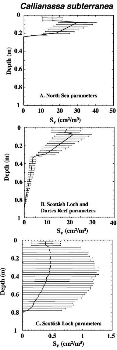
Mesocosm studies of C. subterranea collected from sandy North Sea sediments suggest that these shrimp construct burrows with 5.9 ¡ 1.6 openings at the sediment/water interface connecting to a lattice of nearly horizontal cham-bers.45This complex morphology is approximated in this study
by treating each burrow as a combination of three intersecting
U-shaped burrows (Table 1). This results in a distinct subsur-face maximum in burrow wall sursubsur-face area at approximately 10cm depth (Fig. 3A).
However, C. subterranea burrows do not always resemble intersecting U-shapes. Nickell and Atkinson report several C. subterranea burrow casts from muddy Scottish Loch sediments with single, nearly vertical shafts extending down-ward from a lattice of horizontal tunnels.48 Tudhope and Scoffin found even more complex C. subterranea burrow networks that typically had 5 or more downward-inclined chambers radiating from a central U-shaped burrow.49 To
account for the presence of the deep shafts found in these studies,C. subterraneaburrows are modeled using a combina-tion of 50%U-shaped and 50% Y-shaped burrows (Fig. 3B). The addition of Y-shaped burrows representing deeply penetrating shafts results in the persistence of significant burrow surface area to depths of greater than 80 cm, compared to less than 25 cm in simulations using onlyU-shaped burrows (Fig. 3A,B). However, the deeper portions of Y-shaped Callianassa burrows may be irrigated only infrequently, so that without consideration of flushing frequency the model may lead to overestimates of the bioirrigation intensity at depth.
In muddy subtidal sediments from the west coast of Scotland, Atkinson and Nash found only oneC. subterranea burrow, out of 17 casts, that had more than a single inhalent shaft opening to the surface.46However, Nickell and Atkinson
found that most burrows from this environment had an additional, much smaller exhalent shaft that opened or partially opened at the sediment surface, perhaps facilitating flow of water through the burrows.48 Reported organism densities in these sediments are much lower than estimates from North Sea sites, and burrow depths are considerably greater. To examine the potential differences in surface area resulting from the extremes of reported burrow morphologies, these Scottish Loch burrows are modeled here assuming only a single connection to the surface, by using 50% L-shaped and 50% vertical/45u inclined burrow shapes. This results in a distinct increase in burrow wall surface area at approximately 10 cm, which is not dissimilar from the subsurface maxima resulting from simulations using U- and Y-shaped burrows (Fig. 3C). Thus,C. subterraneais likely to promote deep bioirrigation in all of these settings, with a subsurface maximum in burrow surface area at depths of 10 cm or greater.
Echiura: Bonellidae:Maxmuelleria lankesteri
The echiuran wormMaxmuelleria lankesteri has been recog-nized as an important bioturbator because, unlike many other burrowing macrofauna, it builds extremely deep, temporally persistent burrows. Single burrows have been observed to remain in place for at least 15 months and are suspected to persist in a single location for years.37,38AlthoughM. lankesteri is found from the west coast of Scotland to the Skagerrak, its burrows have been studied particularly in Irish Sea sediments, where the organism is thought to promote deep, rapid mixing of radionuclide contaminants into the sediment.36,37,43
There has been some controversy surrounding the morphol-ogy ofM. lankesteriburrows.35,38In this study, simulations of
a very high variability in irrigation intensity can be expected below 30 cm.
Nereididacea: Nereididae:Nereis diversicolor
The polychaete worm Nereis diversicolor inhabits estuarine, intertidal sediments throughout Europe.40,50–52 Very high population densities (2000–4000 individuals m22
) are com-mon, suggesting that in many estuaries these polychaetes contribute significant bioirrigation intensity. Burrow morphol-ogies have been studied in laboratory mesocosms and field settings using resin casting and X-radiography.40,53Although
burrows have frequently been described as having a simple
U-shape, Davey has shown that in mesocosmsN. diversicolor burrows initiate in aU-shape, but soon exhibit more complex morphologies.40 After several hours, burrows are extended to form a Y-shape, and after several days have complex morphologies including multiple openings at the sediment/ water interface. The morphology ofN. diversicolorburrows in natural sediments may depend on animal population densities;
U-shaped burrowsof N. virensare constructed at low animal densities, but in dense populations burrows may beI-, L- or
Y-shaped.54Although Gerino and Stora describeN. diversicolor burrows in their study asU-shaped,53X-radiographs of these burrows shown in their Fig. 1 suggest that they areY-shaped. X-radiographs of burrows shown in Davey and Gerino and Stora are used to estimate the depths and horizontal extent of burrows (Table 1).40,53 The resulting surface area depth
profile agrees closely with burrow wall surface areas measured
by Gerino and Stora53 using resin casts of 4 individual N. diversicolorburrows from a mesocosm study (Fig. 5).
Decapoda: Ocypodidae:Uca minax,Uca pugnax, andUca pugilator
Fiddler crabs, including the sand fiddler (Uca pugilator), the mud fiddler (Uca pugnax) and the brackish water fiddler (Uca minax) are among the most numerous and conspicuous of burrowing macrofauna in intertidal mangrove and saltmarsh sediments.55–58 Estimates of fiddler crab densities in a
salt-marsh at Sapelo Island, GA are as high as 205¡46 m22
and burrows have been reported to penetrate to depths of up to 65 cm.57,59 However, unlike other burrowing macrofauna, fiddler crabs do not permanently inhabit or actively irrigate their burrows. In fact, some fiddler crabs plug their burrow entrances to prevent flooding during tidal innundation.55,60,61 Fiddler crab burrows are nonetheless likely to contribute to solute transport, because of the abundance of abandoned burrows that are passively flushed by tidal innundation. However, most studies of fiddler crabs report only aperture or organism densities, making an assessment of flushed burrow density difficult.
Burrow network simulations suggest thatU. minaxburrows, because of their large size (Table 1), will contribute most to irrigation, especially at depths greater than 30 cm (Fig. 6C). Simulated burrow wall surface area profiles forU. pugilator and U. pugnax both exhibit a subsurface maximum at approximately 10 cm depth (Fig. 6A,B), with few burrows extending deeper than 20–25 cm into the sediment.
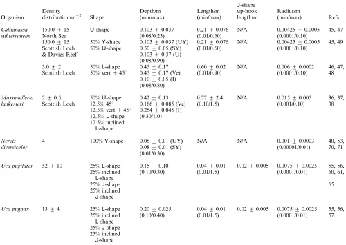
Table 1 Parametrization of burrows. Cumulative distribution functions are Gaussian. Ve~vertical burrow parameter; UY~upper branches of Y-shaped burrow parameter; SY~stem ofU-shaped burrow parameter;I~45uinclined burrow parameter; U~U-shaped burrow parameter; Y~Y-shaped burrow parameter, L~L-shaped burrow parameter
Organism
Density distribution/m22
Shape
Depth/m (min/max)
Length/m (min/max)
J-shape up-hook length/m
Radius/m
(min/max) Refs
Callianassa 150.0¡15 U-shape 0.103¡0.037 0.21¡0.076 N/A 0.00425¡0.0005 45, 47
subterranean North Sea (0.08/0.23) (0.01/0.60) (0.0001/0.10)
150.0¡15 50%Y-shape 0.103¡0.037 (UY) 0.21¡0.076 N/A 0.00425¡0.0005 45, 49 Scottish Loch 50%U-shape 0.50¡0.05 (SY) (0.01/0.60) (0.0001/0.10)
& Davies Reef 0.103¡0.37 (U) (0.08/0.90)
3.0¡2 50%L-shape 0.45¡0.17 0.60¡0.02 N/A 0.006¡0.0002 46, 47, Scottish Loch 50% vert145u 0.45¡0.17 (Ve) (0.01/0.90) (0.0001/0.10) 48
0.10¡0.05 (I) (0.08/0.80)
Maxmuelleria 2¡0.5 50%U-shape 0.42¡0.13 0.77¡2.4 N/A 0.015¡0.005 36, 37,
lankesteri Scottish Loch 12.5% 45u 0.166¡0.085 (Ve) (0.10/1.5) (0.001/0.10) 38
12.5% vert145u 0.254¡0.045 (I) 12.5%L-shape (0.30/1.0) 12.5% inclined
L-shape
Nereis 4 100%Y-shape 0.08¡0.01 (UY) N/A N/A 0.001¡0.0003 40, 53,
diversicolor 0.08¡0.01 (SY) (0.00001/0.01) 70, 71
(0.01/0.30)
Uca pugilator 52¡10 25%L-shape 0.15¡0.10 0.04¡0.01 0.02¡0.005 0.0075¡0.0025 55, 56,
25% inclined L-shape
(0.10/0.30) (0.01/1.5) (0.0001/0.01) 60, 61,
25%J-shape 65
25% inclined J-shape
Uca pugnax 13¡4 25%L-shape 0.20¡0.025 0.04¡0.01 0.02¡0.005 0.0075¡0.0025 55, 56,
25% inclined L-shape
(0.10/0.40) (0.01/1.5) (0.0001/0.01) 57
25%J-shape 25% inclined
Decapoda: Grapsidae:Sesarma reticulatumandEurytium limosum
The marsh crab Sesarma reticulatum occurs in a variety of intertidal marsh environments.55–57,62 Reported population
densities range from 30 m22in levee marshes with tall-form
Spartina alterniflorato just 1 m22in unvegetated creek banks.55
Burrows are extensive and, especially near the sediment
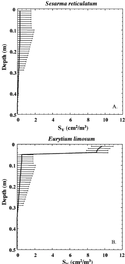
surface, have complex morphologies. Typical burrows have several entrances attaching a shallowly sloping initial tunnel several cm long to the surface. This initial tunnel network is connected to a single vertical shaft of 2–5 cm diameter that descends into the sediment to depths averaging 13–30 cm, although depths of up to 75 cm have been reported.56,62 S. reticulatum burrow networks were simulated in greatly simplified form as single vertical shafts (Table 1). This results in a burrow surface area profile that decays gradually with depth (Fig. 7A).
Another crab species found frequently in both vegetated and unvegetated intertidal saltmarshes is Eurytium limosum.55,57 E. limosumburrows are typically composed of two or more shallow tunnels that extend laterally for 60–70 cm; a single inclined shaft joins the long, shallow tunnels and descends to 20–30 cm depth to create a broadly Y-shaped burrow.57 E. limosumburrows were simulated in this study by treating each burrow as a combination of two shallow, intersecting
L-shaped and one deep 45u-inclined burrows. The presence of just a fewE. limosumburrows greatly enhances burrow surface areas in the upper few centimeters of the sediment column (Fig. 7B).
Fig. 3 Burrow wall surface area per unit sediment volume,SV, as a
function of depth for burrow network simulations of the Thalanassid shrimp Callianassa subterraneausing (A) U-shaped burrows (North Sea site parameters), (B) U- and Y-shaped burrows (North Sea & Davies Reef site parameters) or (C) L-shaped and vertical 1 45u inclined shapes (Scottish Loch site parameters). Data used for all calculations are shown in Table 1.
Fig. 4SVas a function of depth for burrow network simulations of the
Echiuran worm Maxmuelleria lankesteri. Parameters are given in Table 1.
Fig. 5Comparison ofSvfor four individualNereis diversicolorfrom
Gerino and Stora53(solid blue line) and from this study (dotted red
Enteropreusta: Spengelidae:Schizocardium sp.
Laboratory mesocosms have been used to assess the role of the funnel-feeding acorn worm Schizocardium sp. in promoting bioirrigation of shallow, near-shore sediments in St. Louis Bay, Mississippi Sound.32 X-radiographs of mesocosm sediment slabs suggest thatSchizocadium sp.build approximatelyU- or
V-shaped burrows penetrating to a maximum of 9 cm depth. Burrow networks were simulated in this study assuming that all burrows are approximately V-shaped. The resulting surface area profiles decrease continuously with depth (Fig. 8A).
X-radiography of sediment slabs has been used to directly
determine Schizocardium burrow densities as a function of depth in four mesocosms.32The expected depth-dependence of Schizocardiumburrow density, given the animal densities in the various mesocosms (100, 311, 356, 800 m22), is calculated with the stochastic model with parameters given in Table 1 (Fig. 8B). Because total animal densities are known and therefore are kept invariant in the stochastic model, standard deviations shown in Fig. 8B are relatively small. In all four cases, burrow density profiles calculated using the stochastic model are in very good agreement with reported densities from X-radiography of sediment slabs.
Dry Tortugas, Florida, USA
Macrofaunal consortia. The consortium of bioturbating macrofauna present in shallow-water carbonate reef sediments at Dry Tortugas, FL has been described by D’Andrea and Lopez.63 Of the deeply (w4 cm) bioturbating organisms,
D’Andrea and Lopez suggest that the polychaete worm Notomastus sp. (density ~ 113.2 m22) and the burrowing Fig. 6 SVas a function of depth for fiddler crabs including (A)Uca
pugilator, (B)Uca pugnax, and (C)Uca minax. Parameters are given in Table 1.
Fig. 7SV as a function of depth for the mud crabs (A) Sesarma
shrimpCallianassa sp. (density~ 40.8 m22) are dominant.63 Notomastus, a deep deposit feedingcapitellid polychaete, was commonly found at depths greater than 15 cm, most often occurring at 25–30 cm depth.63
To simulate burrow networks at Dry Tortugas, only the dominant deep bioturbators Notomastus andCallianassaare considered here.Notomastusburrows are assumed to be similar in morphology to those of the polychaeteNereis diversicolor, with penetration depths of 20¡2.5 cm forNotomastus. In fact, this is a great simplification;Notomastus burrows have been reported to resemble complex spirals (D’Andrea and Lopez, personal communication), thus, Notomastus burrows may contribute a greater surface area of exchange than is considered here. Callianassa sp. are assumed to build burrows with morphology similar to those reported for Great Barrier Reef Sediments49 and are therefore modeled using the U- and
Y-shapedCallianassaburrow parameters given in Table 1. The presence of these two organisms alone leads to a burrow surface area profile with three distinct regions; in the upper 6 cm surface areas are high and essentially constant with depth, from
6–12 cm they decrease rapidly and then more gradually in the depth interval 12 to 90 cm (Fig. 9A).
Bioirrigation coefficients. From the surface area profiles shown in Fig. 9A, bioirrigation coefficients are calculated using eqn. (6) and (10).Diis calculated using porosity and molecular
Fig. 8 (A)SVas a function of depth for the acorn wormSchizocardium
sp.with mean animal density of 500 m22. (B) Burrow densities for
populations of 100 m22(blue), 311 m22(red), 356 m22(black) and 800 m22(green). Lines are burrow densities from this study; symbols
represent number of active burrows reported from X-radiography of mesocosm slabs.32 Error bars represent ¡1 standard deviation in
burrow density.
Fig. 9(A) SVas a function of depth in shallow carbonate sediment at
Dry Tortugas, FL, USA, from simulations using a consortium of the polychaete wormNotomastus sp.and the shrimpCallianassa sp. (B) Bioirrigation coefficients (s21) as a function of depth for Dry Tortugas, FL derived by fitting an early diagenetic model to measured pore water profiles (Furukawaet al.;32red solid lines), and estimated from the burrow network in this model. Blue line indicatesaO2calculated using
L~2.6 mm from Furukawaet al.,15with eqn. (5), assumingC b~C0.
Green line indicatesaO2corrected forCbusing eqn. (17) and (20). (C)
Bioirrigation coefficients (s21) as a function of depth from Furukawaet
al.32(red lines) and estimated from the burrow network in this model. Blue line indicatesaSO4-2calculated using sulfate concentration and
reduction rate profiles from Furukawaet al.;32green line indicatesaSO4-2
corrected forCbusing eqn. (17) and (20). Orange solid line indicates
diffusion coefficient data given in Furukawaet al.15andr1is
calculated using eqn. (7) with surface areas and burrow densities obtained from the stochastic network simulations. The O2penetration depth at the SWI (LO2) is set to 2.6 mm,
based on vertical microelectrode profiles measured by Furukawaet al.,15 and is used to calculate r¯O2 according to
eqn. (10); values vary from 4.8 to 6.4 mm. At the SWI, this results in predicted irrigation coefficients that are approxi-mately twice as high as the values estimated by Furukawaet al. from diagenetic modeling of chemical data15(Fig. 9B), perhaps reflecting the use ofLO2measured at the SWI, rather than at
the BSI. The predicted irrigation coefficients also exhibit a less pronounced decrease with depth than the coefficients obtained by Furukawaet al.32The higher irrigation coefficients estimated in this study may be due, at least in part, to imperfect burrow flushing. Eqn. (17) and (20) are used to assess this possibility. This correction leads to lower irrigation coeffi-cients, with mean values within a factor of 2 of estimates from Furukawaet al.15Nonethless, the results suggest that O2
gradients measured at the SWI may not yield accurate estimates of radial diffusion length scales at the BSI at depths greater than a few mm.
Bioirrigation coefficients are also calculated by combining the stochastic burrow network simulations with sulfate con-centration and reduction rate profiles taken from Furukawa et al.15The resulting irrigation coefficients predicted using eqn. (6) and (12) are only slightly larger than those predicted by Furukawa et al.15 and exhibit a similar depth-dependence
(Fig. 9C). Because sulfate is a less reactive solute than O2,
correction of this profile for inefficient flushing using eqn. (17) and (20) has negligible effect (Fig. 9C). Both the corrected and uncorrected sulfate bioirrigation coefficient values are sig-nificantly smaller than those calculated for O2. This is primarily
because of the much larger radial diffusion length scales calculated for SO42
2
. Sulfate reactive length scales are also large relative to those obtained from O2microprofiles, because
they are calculated from bulk sulfate reduction rates that decrease rapidly with depth, reflecting changing reactivity with depth.
Bioirrigation coefficient profiles are also calculated here completely independently from data in Furukawaet al.,15by
assuming zero order kinetics for sulfate reduction and using eqn. (16). In this case, the irrigation coefficients, which depend only on the burrow sizes and spacings, are approximately a factor of 3 lower than those calculated by Furukawaet al.15 right at the SWI (Fig. 9C). Below a few mm, however, good agreement between the two independent approaches is observed.
Sapelo island, GA, USA: unvegetated creek bank
Macrofaunal consortia. Intertidal saltmarshes at Sapelo Island, GA are populated by diverse, abundant burrowing macrofauna.55,57,59,64–66Basan and Frey report 1040 burrow apertures m22
in an unvegetated creek bank at Sapelo Island,57 and suggest that the majority of these apertures are due to polychaete worms includingNereis succineaandHeteromastus filiformus. Other burrows are attributed to fiddler crabs, especiallyUca pugilator, burrowing shrimp includingUpogebia affinis and predatory mud crabs such as Panopeus herbsti, which share the burrows of Sesarma reticulatum.56Teal also
inventoried burrowing macrofauna at an unvegetated creek bank on Sapelo Island, GA and foundUca pugilator(52 m22), Uca pugnax (13 m22), Sesarma reticulatum (1 m22) and
Eurytium limsosum(6 m22
).55
A simulated burrow network for an unvegetated creek bank at Sapelo Island, GA was completed using U. pugilator, U. pugnaxandE. limosumdensities taken directly from Teal,55 while forS. reticulatumandP. herbstiaverages of data given forS. reticulatumby Teal and forP. herbstiby Basan and Frey
are used.55,57Upogebia affinisshrimp burrows are assumed to be similar in morphology toCallianassashrimp. A polychaete density of 450¡50m22
is derived by assuming a total aperture density of y1000 m22 of which y100 m22 are due to organisms other than polychaetes.
Burrow wall surface areas for polychaetes, shrimp and fiddler crabs only are highest near the sediment-water interface and decay gradually to a depth of approximately 30 cm (Fig. 10A). The addition of E. limosum/P. herbsti burrows results in much higher burrow wall surface areas in the upper few cm of sediment and a more rapid decay of the burrow surface areas with depth (Fig. 10B).
Bioirrigation coefficients. As for the Dry Tortugas site, the stochastic model-derived surface areas shown in Fig. 10B are used with eqn. (6) and (10) to derive a bioirrigation coefficient profile. A porosity of 76%67is used to obtainDO2, andr1is
calculated using eqn. (7). Using a measured O2 flux of 68–
89 mmol O2m22d21yields O2penetration depth (LO2) values
between approximately 0.2 mm and 1.0 mm.72Given that the marsh sediments are periodically exposed to the atmosphere, anLO2value of 1.0 mm is used in this study, which results inr¯O2
values that vary from 4.1 to 17.0 mm. The resulting bioirrigation coefficient profile, shown in Fig. 10C, is compared to that of Meileet al.68who used an inverse modeling approach to obtain a bioirrigation coefficient profiles from sulfate concentration and reduction rate measurements. In the upper 5 cm of sediment, bioirrigation coefficients from this study are approximately a factor of 2 greater than those of Meileet al.,68 and the bioirrigation coefficient profile from this study does not decay as rapidly with depth. Eqn. (17) and (20) are used to correct the profile for the effects of imperfect burrow flushing. The resulting profile still suggests more intense irrigation throughout the sediment than the profile of Meileet al.68
The lower irrigation values given by Meileet al.68may reflect differences in solute-specific irrigation coefficients. Therefore, irrigation coefficients for sulfate are calculated here using sulfate concentration and reduction rate profiles67,68and eqn. (6) and (12). The resulting irrigation coefficient profile (Fig. 10D) is in excellent agreement with the profile given by Meileet al.68Correction of the stochastically-derived bioirriga-tion coefficients for the effects of imperfect flushing using eqn. (17) and (20) does not significantly change the profile.
Bioirrigation coefficients are also calculated assuming zero order kinetics for sulfate reduction. The resulting profile, which depends only on the burrow sizes and spacings, and which is completely independent from the sulfate concentration and reduction rate profiles used by Meileet al.,68is also shown in Fig. 10D. The resulting bioirrigation coefficients are somewhat smaller than those of Meileet al.68Overall, the results for the
creek bank sites indicate that it is possible to obtain meaningful irrigation coefficients from the stochastically simulated burrow network.
Sapelo island, GA, USA: vegetated ponded mash
Macrofaunal consortia. The abundance and composition of macrofaunal communities present in saltmarsh environments shows significant spatial zonation, with community composi-tion depending on length of tidal innundacomposi-tion, presence or absence of vegetation and sediment composition.57Thus, areas
of the marsh with dense, diverse macrofaunal populations, such as the unvegetated creek bank discussed above, are likely to have deeper, more intense bioirrigation than regions of the marsh with fewer organisms. For example, ponded marsh regions are much more sparsely populated with macrofauna than creek bank sites. At Sapelo Island, GA, Basan and Frey reporty415 burrow apertures m22
crab Uca pugnax(27 ¡7 m22) and the mud crab Eurytium limosum (4 ¡ 1 m22).55 All other burrow apertures (y280
m22
) are likely due to the polychaete worm Nereis succinea. Basan and Frey report that burrow depths are typically shorter in the densely vegetated ponded marsh,57 and that burrow
shapes are typically less complex. In simulations,Uca pugnax burrows at the ponded marsh were assumed to reach a mean depth of only 15 cm, compared to 20 cm at the creek bank. The lower density of organisms inhabiting the ponded marsh leads to lower surface areas as a function of depth compared to the creek bank site (Fig. 11A).
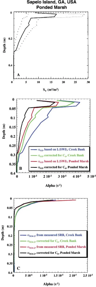
Bioirrigation coefficients. Bioirrigation profiles at the ponded marsh are calculated for both dissolved O2 and
SO42 2
. O2irrigation coefficient profiles are calculated using a
vertical diffusion length scale of 1.0 mm, as for the creek bank site. Diffusion coefficients were corrected using the porosity of 85% reported by Kostkaet al.67 Dissolved SO42
2
irrigation coefficient profiles are calculated using measured sulfate concentration and reduction rate profiles.67,69Correction for inefficient burrow flushing results in slightly lower O2irrigation
coefficients, but has no significant impact on SO422irrigation
coefficients (Fig. 11B, C). The intensity of irrigation, especially as indicated by the O2irrigation coefficient profiles is somewhat
less than at the creek bank site. The depth of irrigation is also somewhat shallower at the ponded marsh, because of the lower density of deep-burrowing infauna and because infauna in ponded marsh areas tend to build shallower burrows than in creek bank sediments.57 Because of shallower irrigation, the ponded marsh sediments have a more compressed redox stratification, with more reducing conditions closer to the sediment surface, compared to the more intensely irrigated creek bank sediments.69
Comparison of diagenetic and stochastic irrigation models
Model results obtained at Dry Tortugas, FL and Sapelo Island, GA demonstrate that the ecologically-based stochastic model yields bioirrigation coefficients that are comparable to those obtained independently via inverse modeling or by use of multicomponent early diagenetic reactive transport models. The latter do not require information concerning the benthic organisms responsible for irrigation, rather, bioirrigation coefficients are inferred from model simulations fitting measured chemical and/or reaction rate profiles (Meileet al., 2001). In contrast, the stochastic model presented here explicitly uses ecological data to calculate irrigation intensities. Pore water profiles are notper serequired, although the radial diffusive length scale (L) across the burrow-sediment interface must be specified. As few direct measurements of L are currently available,Lvalues are constrained here using other available chemical data.
An important strength of the stochastic model is that uncertainties associated with calculated bioirrigation intensities can be evaluated. The uncertainties derive from the probability density functions describing the burrow network, which in turn are based on statistical information about the ecological variables (animal density, burrow size and geometry). Thus, the model-calculated uncertainties on the bioirrigation coefficients
Fig. 10(A) SV as a function of depth in an unvegetated saltmarsh
creekbank at Sapelo Island, GA, USA including polychaete worms, fiddler crabs and the mudcrabsSesarma reticulatum and Panopeus herbsterii. (B)SV(cm2/m3) with all of the organisms included in (A) as
well as Eurytium limosum. (C) Bioirrigation coefficients (s21) as a
function of depth calculated using inverse modeling of chemical data (red solid line)68anda
O2estimated from the burrow network in this
model usingL~1.0 mm with eqn. (6), assumingCb~C0(blue solid
line) and with correction for depletion of O2within burrows (green
line). (D)aSO4-2bioirrigation coefficients calculated using the stochastic
network model with measured sulfate reduction rates, without correction forCb(blue line) and with correction forCb(green line).
reflect the natural variation in abundance and burrowing activity of the benthic macrofauna.
The stochastic model is not intended to replace early reactive transport models of early diagenesis. Rather, it is an additional tool to constrain irrigation coefficients, which can then be used in early diagenetic modeling. Independent estimates of trans-port parameters significantly enhance the reliability of reactive transport calculations applied to the complex biogeochemical dynamics of sediments.
Conclusions
Aquatic sediments are typically redox stratified, with increas-ingly reducing conditions encountered at depth. However, burrow networks built by macroinfauna create a complex 3-dimensional patchwork of relatively more oxidized or reduced sediment compartments. The resulting increase in interfacial area separating zones with disparate redox characteristics enhances diffusive exchange and creates ecological and geochemical microzones that affect sediment biogeochemical dynamics.
In this study, the spatial distribution of distinct sediment zones due to burrowing macroinfauna are quantified by simu-lating 3D burrow networks for a variety of model organisms and for consortia of organisms in shallow carbonate and intertidal saltmarsh sediments. The conceptual approach provides a link between the ecological characteristics of burrowing macroinfauna and the resulting biogeochemical consequence on solute transport and biogeochemical cycling. The impact on diffusional exchange of solutes between burrow water and bulk sediment is addressed, and quantitative estimates for nonlocal transport parameters are proposed. This is of particular importance, because a quantitative des-cription of biogeochemical dynamics in sediments, for example based on the interpretation of chemical profiles, requires the quantification of transport intensities.
The approach outlined here allows an independent, ecolo-gically-based, assessment of the depth-dependence of bioirriga-tion coefficient profiles. Burrow network simulabioirriga-tions of even relatively simple model organisms are found to result in depth-dependent burrow wall surface areas that are neither constant nor exponentially decreasing over a given interval, as is commonly assumed in bioirrigation models. Network simula-tions of the burrowing shrimp Callianassa subterranea, the echiuran wormMaxmuelleria lankesteri, and the fiddler crab Uca pugilator all result in burrow wall surface areas characterized by a subsurface maximum. These maxima are similar to subsurface maxima in bioirrigation intensity reported in chemically-based studies that have not imposed a priorirestrictions on the depth-dependence of bioirrigation intensity.27,68 Furthermore, model simulations demonstrate that relatively rare organisms may have a disproportionate influence on solute transport in sediments. For example, burrow wall surface area profiles calculated for an unvegetated saltmarsh creek bank site at Sapelo Island, GA with and without the mud crabE. limosumare quite distinct (Fig. 10A,B), in spite of the fact thatE. limosum, is responsible for only 6 out ofy1000 apertures m22.
Burrow network simulations provide estimates of burrow surface areas as a function of depth, which are used to derive nonlocal bioirrigation coefficients. In carbonate reef sediments at Dry Tortugas, O2based bioirrigation coefficients calculated
using the stochastic model are somewhat larger than values found through diagenetic modeling.15 However, if the irriga-tion coefficients are corrected for inefficient flushing, using an estimate of the time-averaged value of Cb, the agreement is
better.
Sulfate bioirrigation coefficient profiles calculated using the stochastic model for an unvegetated intertidal saltmarsh creek Fig. 11(A)SVas a function of depth for the ponded marsh (solid line)
sites at Sapelo Island, GA with dotted lines indicating¡1 standard deviation of the surface area. (B) Bioirrigation coefficients (s21) as a
function of depth at Sapelo Island calculated for dissolved O2at the
creek bank (green) or ponded marsh (black) with correction for solute depletion within burrows and without correction for solute depletion at the creek bank (blue) and ponded marsh (purple). (C) Bioirrigation coefficients (s21) as a function of depth at Sapelo Island calculated for dissolved SO422with correction for solute depletion within burrows at
bank site are in good agreement with nonlocal bioirrigation coefficient profiles determined by Meileet al.68using an inverse
modeling approach. Calculated irrigation coefficients for an adjacent ponded marsh site are somewhat lower. This lower mixing intensity may contribute to the more compressed vertical redox zonation observed in chemical pore water profiles at the ponded marsh compared to the creek bank.69
To go beyond the model presented here, further information is required regarding the depth-dependence of solute concen-trations within burrows, as well as the temporal variation of solute concentrations within burrows. Nonetheless, the current model provides an extremely useful link between benthic macrofaunal ecology and a quantitative description of chemical transport by bioirrigation.
Acknowledgement
We would especially like to thank Yoko Furukawa, Dawn Lavoie and Sam Bentley for discussions of the work presented here and for providing us with benthic mesocosm data. The comments of two anonymous reviewers are appreciated and helped to improve this manuscript. This research was supported by Office of Naval Research grants N00014-98-1-0203 and N00014-01-0599 and the Netherlands Organisation of Scientific Research (NWO-Pionier programme). Acknow-ledgement is made to the Office of Naval Research Biomole-cular and Biosystems S&T Division for support of travel to the symposium resulting in the present special volume.
References
1 R. C. Aller,Geochim. Cosmochim. Acta, 1980,44, 1955–1965. 2 R. C. Aller,Geochim. Cosmochim. Acta, 1984,48, 1929–1934. 3 R. C. Aller and J. Y. Aller,J. Mar. Res., 1998,56, 905–936. 4 G. Matisoff, J. B. Fisher and S. Matis,Hydrobiologia, 1985,122,
19–33.
5 B. P. Boudreau and R. L. Marinelli,J. Mar. Res., 1994,52, 947– 968.
6 R. C. Aller, J. Y. Yingst and W. J. Ullman,J. Mar. Res., 1983,41, 5671–604.
7 D. M. Alongi,Mar. Ecol.: Prog. Ser., 1985,23, 207–208. 8 G. M. Branch and A. Pringle,J. Exp. Mar. Biol. Ecol., 1987,107,
219–235.
9 F. C. Dobbs and J. B. Guckert,Mar. Ecol.: Prog. Ser., 1988,45, 69–79.
10 N. P. Revsbech, J. Sørensen, T. H. Blackburn and J. P. Lomholt,
Limnol. Oceanogr., 1980,25, 403–411.
11 W. M. Smethie, Jr., C. A. Nittrouer and R. F. L. Self,Mar. Geol., 1981,42, 173–200.
12 D. E. Hammond, C. Fuller, D. Harmon, B. Hartman, M. Korosc, L. G. Miller, R. Rea, S. Warren, W. Berelson and S. W. Hager,
Hydrobiologia, 1985,129, 69–90.
13 Y. Wang and P. Van Cappellen,Geochim. Cosmochim. Acta, 1996, 60, 2993–3014.
14 H. Fossing, T. G. Ferdelman and P. Berg,Geochim. Cosmochim. Acta, 2000,64, 897–910.
15 Y. Furukawa, S. J. Bentley, A. M. Shiller, D. L. Lavoie and P. Van Cappellen,J. Mar. Res., 2000,58, 493–522.
16 M. B. Goldhaber, R. C. Aller, J. K. Cochran, J. K. Rosenfeld, C. S. Martens and R. A. Berner,Am. J. Sci., 1977,277, 193–237. 17 D. R. Schink and J. N. L. Guinasso,Mar. Geol., 1977,23, 133–
154.
18 D. R. Schink and J. N. L. Guinasso,Am. J. Sci., 1978,278, 687– 702.
19 R. C. Aller, The effects of animal-sediment interactions on geochemical processes near the sediment-water interface, in
Estuarine Interactions, ed. M. L. Wiley, Academic Press, New York, NY, 1978, pp. 157–172.
20 G. Matisoff and X. Wang,Limnol. Oceanogr., 1998,43, 1487– 1499.
21 B. P. Boudreau,Am. J. Sci., 1986,286, 161–198.
22 D. E. Hammond and C. Fuller,The use of radon-222 to estimate benthic exchange and atmospheric exchanges in San Francisco Bay, ed. T. J. Conomos, San Francisco Bay: the Urbanized Estuary, Pacific Div. Am. Ass. Adv. Sci, San Francisco, 1979, pp. 213–230. 23 R. J. McCaffrey, A. C. Myers, E. Davey, G. Morrison, M. Bender,
N. Luedte, D. Cullen, P. Froelich and G. Klinkhammer,Limnol. Oceanogr., 1980,25, 31–44.
24 B. P. Boudreau,American Journal of Science, 1986,286, 199–238. 25 B. P. Boudreau and D. M. Imboden,Am. J. Sci., 1986,286, 693–
719.
26 S. Emerson, R. Jahnke and D. Heggie,J. Mar. Res., 1984,42, 709– 730.
27 J. P. Christensen, A. H. Devol and W. M. Smethie, Jr.,Cont. Shelf Res., 1984,3, 9–23.
28 B. P. Boudreau,J. Mar. Res., 1984,42, 731–735.
29 W. R. Martin and G. T. Banta,J. Mar. Res., 1992,50, 125–154. 30 M. Schlu¨ter, E. Sauter, H.-P. Hansen and E. Suess, Geochim.
Cosmochim. Acta, 2000,64, 821–834.
31 P. Van Cappellen and J.-F. Gaillard, Biogeochemical dynamics in aquatic sediments, in Reactive transport in porous media, ed. P. C. Lichtner, C. I. Steefel and E. H. Oelkers, 1996, Mineralogy Society of America, Washington DC, pp. 335–376.
32 Y. Furukawa, S. J. Bentley and D. L. Lavoie,J. Mar. Res., 2001, 59, 417–452.
33 R. C. Aller and J. Y. Yingst,J. Mar. Res., 1985,43, 615–645. 34 E. A. Shinn,J. Paleontol., 1968,42, 879–894.
35 D. J. Hughes, A. D. Ansell and R. J. A. Atkinson,J. Exp. Mar. Biol. Ecol., 1996,195, 203–220.
36 D. J. Hughes, A. D. Ansell, R. J. A. Atkinson and L. A. ,J. Nat. Hist., 1993,27, 219–248.
37 L. A. Nickell, R. J. A. Atkinson, D. J. Hughes, A. D. Ansell and C. J. Smith,J. Nat. Hist., 1994,29, 871–885.
38 D. J. Hughes, R. J. A. Atkinson and A. D. Ansell,J. Exp. Mar. Biol. Ecol., 1999,238, 209–223.
39 J. D. Howard,Sedimentology, 1969,11, 249–258. 40 J. T. Davey,J. Exp. Mar. Biol. Ecol., 1994,179, 115–129. 41 RJ. A. Atkinson and R. D. M. Nash,Prog. Underwater Sci., 1985,
10, 109–115.
42 R. J. A. Atkinson,Proc. R. Soc. Edinburgh, 1986,90B, 351–361. 43 D. J. Hughes and R. J. A. Atkinson,J. Mar. Biol. Assoc. UK, 1997,
77, 635–653.
44 R. Witbaard and G. C. A. Duineveld,Sarsia, 1989,74, 209–219. 45 A. A. Rowden and M. B. Jones,J. Nat. Hist., 1995,29, 1155–1165. 46 R. J. A. Atkinson and R. D. M. Nash,J. Nat. Hist., 1990,24, 403–
413.
47 R. B. Griffis and T. H. Suchanek,Mar. Ecol.: Prog. Ser., 1991,79, 171–183.
48 L. A. Nickell, D. J. Hughes and R. J. A. Atkinson, Megafaunal bioturbation in organically enriched Scottish sea lochs, Biology and Ecology of Shallow Coastal Waters: Proceedings of the 28th European Marine Biology Symposium, Herakleion, Greece, Olsen and Olsen, Frendensborg, International Symposium Series, 1995. 49 A. W. Tudhope and T. P. Scoffin,J. Sed. Petrol., 1984,54, 1091–
1096.
50 E. Kristensen,Holarct. Ecol., 1984,7, 249–256.
51 J. T. Davey and C. L. George,Est. Coast. Shelf Sci., 1986,22, 603– 618.
52 M. Nithart,J. Mar. Biol. Assoc. UK, 1998,78, 131–143. 53 M. Gerino and G. Stora,Comptes Rendus Acad. Sci. Paris, 1991,
313, 489–494.
54 G. Miron, G. Desrosiers, C. Retiere and R. Lambert,Can. J. Zool., 1991,69, 39–42.
55 J. M. Teal,Ecology, 1958,39, 185–193.
56 E. A. Allen and H. A. Curran,J. Sedim. Petrol., 1974,44, 538–548. 57 P. B. Basan and R. W. Frey, Actual-paleontology and neoichnol-ogy of salt marshes near Sapelo Island, Georgia, inTrace Fossils 2, ed. T. P. Crimes and J. C. Harper, Steel House Press, London, 1977, pp. 41–70.
58 D. M. Alongi, Mangroves and salt marshes, inCoastal Ecosystem Processes, CRC Press, New York, 1998, pp. 43–92.
59 P. L. Wolf, S. F. Shanholtzer and R. J. Reimold,Crustaceana, 1975,91, 79–91.
60 J. B. Dembowski,Biol. Bull., 1926,50, 179–201. 61 J. H. Christy,Animal Behav., 1982,30, 687–694. 62 O. W. Crichton,Est. Bull., 1960,5, 3–10.
63 A. F. D’Andrea and G. R. Lopez,Geo-Mar. Lett., 1997,17, 276– 282.
64 J. M. Teal,Ecology, 1962,43, 614–624.
65 R. W. Frey and T. V. Mayou,Senckenbergiana maritima, 1971,3, 53–77.
66 C. L. Montague, The influence of fiddler crab burrows and burrowing on metabolic proceses in salt marsh sediments, in
Estuarine Comparisons, ed. V. S. Kennedy, 1982, Academic Press, New York, pp. 283–301.
temporal gradients in saltmarsh sediments, 2001,Biogeochemistry, in press.
68 C. Meile, C. M. Koretsky and P. Van Cappellen, Limnol. Oceanogr., 2001,46, 164–177.
69 C. M. Koretsky, P. Van Cappellen, T. J. DiChristina, J. E. Kostka, K. L. Lowe, C. Moore, A. N. Roychoudhury and E. Viollier, Contrasting geochemical and microbial structures of saltmarsh
sediments: seasonal and spatial trends at Sapelo Island (Georgia, USA), in preparation.
70 M. Emmerson,Helgoland Mar. Res., 2000,54, 110–116. 71 V. F. Clavero, F. X. Niell and J. A. Fernandez,Est. Coast. Shelf
Sci., 1991,33, 193–202.