Bivariate beta-generated distributions with applications to well-being data

(1)

R E S E A R C H

Open Access

Bivariate beta-generated distributions with

applications to well-being data

José María Sarabia

*

, Faustino Prieto and Vanesa Jordá

*Correspondence: [email protected] Department of Economics, University of Cantabria, Avda. de los Castros s/n, 39005 Santander, Spain

Abstract

The class of beta-generated distributions (Commun. Stat. Theory Methods 31:497–512, 2002; TEST 13:1–43, 2004) has received a lot of attention in the last years. In this paper, three new classes of bivariate beta-generated distributions are proposed. These classes are constructed using three different definitions of bivariate distributions with classical beta marginals and different covariance structures. We work with the bivariate beta distributions proposed in (J. Educ. Stat. 7:271–294, 1982; Metrika 54:215–231, 2001; Stat. Probability Lett. 62:407–412, 2003) for the first proposal, in (Stat. Methods Appl. 18: 465–481, 2009) for the second proposal and (J. Multivariate Anal. 102:1194–1202, 2011) for the third one. In each of these three classes, the main properties are studied. Some specific bivariate beta-generated distributions are studied. Finally, some empirical applications with well-being data are presented.

Mathematics Subject Classification (2000): 62E15; 60E05

Keywords: Classical beta distribution; Bivariate beta distribution; Covariance structure; GB1 and GB2 distributions

1 Introduction

In the recent statistical literature several methodologies of constructing bivariate and multivariate distributions based on marginal and conditional distributions have been proposed; see the works by Arnold et al. (1999; 2001), Kotz et al. (2000), Sarabia and Gómez-Déniz (2008) and Balakrishnan and Lai (2009) among others.

An important field of research focuses on the study of new classes of univariate distri-butions which contain the classical proposals, also allowing for more flexibility in fitting data. In this sense, the class of beta-generated (BG) distributions (Eugene et al. 2002; Jones 2004) has received an increasing amount of attention in recent years.

There are several reasons for studying classes of multivariate beta generated dis-tributions. The two existing proposals of multivariate BG distributions present some drawbacks. The first proposal (Jones and Larsen 2004) is only valid for modeling data above the diagonal. The second proposal (Arnold et al. 2006) is defined in terms of the conditional distributions, and the corresponding marginal distributions do not follow, in general, beta generated distributions.

The three bivariate and multivariate models proposed in this paper present BG marginals, with high flexibility in the marginals and in the dependence structure. The

(2)

marginal distributions of the first model share one of the shape parameters, and the struc-ture of dependence satisfies TP2 condition (see Section 3). The marginals of the second model are free, and the different pairwise of marginals are associated (see Section 3). The third model is the more flexible, in the sense than all the marginals are free (they do not share any shape parameter) and the covariance structure admits correlations of any sign.

On the other hand, these classes of distributions present several fields of applicability. For example, bivariate beta generated distributions with classical beta marginals are nat-ural choices to be used as prior distributions for the parameters of correlated binomial random variables (with any sign for the correlation) in Bayesian analysis (see Apostolakis and Moieni 1987; Arnold and Ng 2011).

In this work, three new classes of bivariate BG distributions are proposed. These classes are constructed using three alternative definitions of bivariate distributions with classical beta marginals and different covariance structures. We work with the bivariate beta dis-tributions proposed by Libby and Novick (1982), Jones (2001) and Olkin and Liu (2003) for the first proposal, El-Bassiouny and Jones (2009) for the second proposal and Arnold and Ng (2011) for the third one. For each of these three classes, the main properties are obtained. Some specific bivariate BG distributions are studied. Finally, some empirical applications with well-being data are presented.

The contents of this paper are as follows. In Section 2 we present some basic properties of the class of the BG distributions and a brief review about two multivariate extensions of the BG distribution. Section 3 considers and studies the three classes of bivariate BG distributions and their main properties as well as to introduce three specific bivariate distributions. A number of applications of these distributions to fit well-being data are presented in Section 4. Finally, some conclusions and future research directions are given in Section 5.

2 Some univariate and multivariate beta-generated distributions

2.1 The univariate class of beta-generated distributions

In this section we present basic properties of the class of BG distributions. We begin with an initial baseline probability density function (PDF)f(x), where the correspond-ing cumulative distribution function (CDF) is represented by F(x). The class of BG distributions is defined in terms of the PDF by (a,b>0),

gF(x;a,b)=[B(a,b)]−1f(x)F(x)a−1[1−F(x)]b−1, (1)

where B(a,b) = (a)(b)/ (a +b) denotes the classical beta function. A random variableXwith PDF (1) will be denoted byX∼BG(a,b;F).

The CDF associated to (1) is,

GF(x;a,b)=IF(x)(a,b),

whereIF(x)(·,·)denotes the incomplete beta ratio.

IfB∼ Be(a,b)represents the classical beta distribution, a simple stochastic represen-tation of (1) is,

(3)

This representation permits a direct simulation of the values of a random variable with PDF (1), which can be also used for generating multivariate versions of the BG distribution. The raw moments of a BG distribution can be obtained by,

EXr=EF−1(B)r

, r>0.

An important number of new classes of distributions have been proposed using this methodology. Some representatives examples of BG distributions include the generalized beta of the first kind (GB1) proposed by McDonald (1984), the generalized beta of the second kind (GB2) proposed and studied by Venter (1983) and McDonald (1984), the logFdistribution (Barndorff-Nielsen et al. 1982), the beta-normal distribution (Eugene et al. 2002), the beta-exponential distribution (Nadarajah and Kotz 2006) and the Skew-t distribution (Jones 2004).

Some extensions of this family have been proposed by Alexander and Sarabia (2010), Alexander et al. (2012), Cordeiro and de Castro (2011) and Zografos (2011). Other alter-native flexible families of distributions can be found in Alzaatreh et al. (2013, 2014) and Lee et al. (2013).

Ifa = iandb = n−i+1 in (1), we obtain the PDF of thei-th order statistic fromF (Jones 2004). Below, we highlight some representative values ofaandb,

• Ifa=b=1,gF=f.

• Ifa=nandb=1, we obtain the distribution of the maximum. • Ifa=1andb=n, we obtain the distribution of the minimum. • Ifa=b, we obtain a family of skew distributions.

Parametersaandbcontrol the tailweight of the distribution. Specifically, theaparameter controls left-hand tailweight and thebparameter controls the right-hand tailweight of the distribution. On the other hand,a= byields a symmetric sub-family, withacontrolling tailweight. Ifa= b= 1 the BG family is always symmetric if the baseline functionF(x)

is symmetric. In this sense, the BG distribution accommodates several kind of tails. For example (see Jones 2004),

• Potential tails: Iff ∼x−(α+1)_and_{α >}_{0, when}_x_{→ ∞}_g

F ∼x−bα−1, • Exponential tails: Iff ∼e−αx_and_{β >}_{0, then}_g

F ∼e−bβxifx→ ∞.

2.2 Two previous classes of multivariate extensions of beta-generated distributions

There are two proposals for multivariate extensions of BG distributions. The first pro-posal used the joint PDF of a subset of order statistics, and has been proposed by Jones and Larsen (2004). The second proposal used the so called Rosenblatt construction (Rosenblatt 1952), and has been proposed by Arnold et al. (2006). These two alternatives are not related with the multivariate BG distributions studied in this paper.

3 Three classes of bivariate beta-generated distributions

(4)

random variable distributed as the classical gamma denoted by X ∼ Ga, with PDF f(x)=[(a)]−1xa−1e−x, withx≥0 anda>0. Then, ifX1∼GaandX2∼Gbare inde-pendent gamma random variables, the transformed random variableX= X1/(X1+X2)

is distributed as the classical beta distribution with parameters(a,b).

3.1 The first class of bivariate beta-generated distributions

The first class of bivariate beta-generated distribution is based on the following class of bivariate beta distribution.

Definition 1.LetGa1,Ga2andGbbe three independent gamma random variables with a1,a2,b > 0. The first class of bivariate beta distribution is defined by the stochastic

representation,

(Z1,Z2)=

Ga1 Ga1+Gb

, Ga2 Ga2+Gb

. (3)

This class was initially proposed by Libby and Novick (1982) and then studied by Jones (2001) and Olkin and Liu (2003).

Now, using (3) we define the following class of bivariate BG distributions.

Definition 2.LetGa1,Ga2andGbbe three independent gamma random variables with a1,a2,b > 0. The first class of bivariate BG distribution is defined by the stochastic

representation,

(X1,X2)=

F₁−1

Ga1 Ga1+Gb

,F₂−1

Ga2 Ga2+Gb

, (4)

whereF1(·),F2(·)are genuine CDF.

3.1.1 Basic properties

In this section we study some basic properties of the bivariate BG distribution defined in (4). The marginal distributions of (4) are BG distributions,

X1 ∼ BG(a1,b;F1),

X2 ∼ BG(a2,b;F2).

Note that both marginals share the second shape parameterb. However, this fact does not make the model less flexible, since both baseline distributionsF1andF2are different.

Using the joint PDF of the bivariate beta distribution (3) (See Appendix), we obtain the joint PDF of the first class of bivariate BG distribution given by,

f(x1,x2)=

F1(x1)a1−1F2(x2)a2−1[1−F1(x1)]a2+b−1[1−F2(x2)]a1+b−1f1(x1)f2(x2)

B(a1,a2,b)[1−F1(x1)F2(x2)]a1+a2+b

,

(5)

wherea1,a2,b > 0 andB(a1,a2,b) = (a1)(a2)(b)/ (a1+a2+b). An alternative

expression of (5) in terms of the PDF of the BG distribution is,

f(x1,x2)=

(a1+b) (a2+b) (b) (a1+a2+b)

gF1(x1;a1,a2+b)gF2(x2;a2,a1+b)

[1−F1(x1)F2(x2)]a1+a2+b

(5)

wheregF(x;a,b)represents the PDF defined in (1). The joint PDF can be also written as an infinite mixture,

f(x1,x2)= ∞

j=0

dA(j)gF1

x1;a1+j,a2+b

·gF2

x2;a2+j,a1+b

, (6)

whered= (a1+b)(a2+b) (b)(a1+a2+b)and

A(j)=

a1+j

(a1) ·

a2+j

(a2) ·

(a1+a2+b) a1+a2+b+j

· 1 j!.

The conditional distribution ofX1givenX2is,

f(x1|x2)=

(a1+a2+b) (a1) (a2) (b)

F1(x1)a1−1[1−F1(x1)]a2+b−1[1−F2(x2)]a1f1(x1)

[1−F1(x1)F2(x2)]a1+a2+b

,

and the regression function ofX1givenX2is,

E(X1|X2=x2)=

(a1+a2+b) (a1) (a2) (b)

(1−F2(x2))a2

1

0

F₁−1(t)ta1−1₍₁−_t₎a2+b−1

[1−tF2(x2)]a1+a2+b

dt.

In order to study the dependence betweenX1andX2, we consider the local dependence

function defined by (Holland and Wang 1987),

γ (x1,x2)= ∂2 ∂x1∂x2

log f(x1,x2).

We use the definitions of total positivity of order 2(TP2)functions and reverse rule of

order 2(RR2)functions, which are the following.

Definition 3.A joint PDFf(x,y)is said to beTP2(RR2) if

f(x,y)f(u,v)−f(x,v)f(u,y)≥0 (≤0)

for allx≤uandy≤v.

The following result relates the local dependence functionγ (x1,x2)with theTP2and

RR2(see Theorem 7.1 in Holland and Wang 1987).

Theorem 1.Letf(x1,x2)be the joint PDF of(X1,X2)with support on a setSwhere the

setS=S1×S2. Then,f(x1,x2)isTP2(RR2) if and only ifγ (x1,x2)≥0(≤0).

For the first class of BG distribution, it can be verified that

γ (x1,x2)=

(a1+a2+b)f1(x1)f2(x2)

[1−F1(x1)F1(x1)]2

>0,

and thenX1andX2areTP2. As a consequence, the linear correlation coefficient between

X1andX2is always positive.

It can be proved (see Shaked 1977) that if the joint PDFf(x1,x2)isTP2(RR2), then the

conditional hazard rate ofX1|X2=x2is decreasing (increasing) inx2. A similar property

holds for the other conditional distributionX2|X1 = x1. As the PDF in (5) isTP2, this

property shows the monotonicity properties of the hazard rate functions of the condi-tional distributions ofX1|X2 = x2as a function ofx2and theX2|X1 = x1as a function

(6)

On the other hand, becauseX1andX2are increasing functions of independent random

variables,X1andX2are associated random variables (Esary et al. 1967).

Expressions for the cross momentsEXr1

1X

r2

2

can be obtained from (5) or in terms of an infinite mixture from (6). On the other hand, ifb>r, it can be shown that,

E

F1(X1)rF2(X2)r

[1−F1(X1)F2(X2)]r

= (a1+r) (a2+r) (b−r) (a1+a2+b) (a1) (a2) (b) (a1+a2+b+r)

.

3.1.2 Extension to higher dimensions

The extension to higher dimensions is direct. The m-dimensional random vector is defined as,

(X1,. . .,Xm)=

F_i−1

Gai

Gai+Gb

,i=1, 2,. . .,m

. (7)

The marginal distributions areXi∼ BG(ai,b;Fi),i =1, 2,. . .,m. The joint PDF of (7) is given by,

f(x1,. . .,xm)=c m

i=1

Fi(xi)ai−1fi(xi) [1−Fi(xi)]ai+1

1+ m

i=1

Fi(xi) 1−Fi(xi)

−b ,

wherec−1=B(a1,. . .,am,b)=(a1)· · ·(am)(b)/ (a1+. . .+am+b).

3.2 The second type of bivariate beta-generated distributions

The second type of bivariate BG distribution is motivated by the fact of having a bivariate distribution with arbitrary BG marginals. This second class is based on the following class of bivariate beta distribution, which was proposed by El-Bassiouny and Jones (2009).

Definition 4.LetGai, i = 1, 2, 3, 4 be independent gamma random variables, where

ai > 0,i = 1, 2, 3, 4. The second class of bivariate beta distribution is defined by the stochastic representation,

(Z1,Z2)=

Ga1 Ga1+Ga3

, Ga2

Ga2 +Ga3+Ga4

. (8)

Now, we define the second class of BG distributions.

Definition 5.LetGai, i = 1, 2, 3, 4 be independent gamma random variables, where

ai > 0,i = 1, 2, 3, 4. The second class of bivariate BG distribution is defined by the stochastic representation,

(X1,X2)=

F₁−1

Ga1 Ga1+Ga3

,F₂−1

Ga2 Ga2 +Ga3+Ga4

, (9)

The marginal distributions are BG distributions with arbitrary parameters,

X1 ∼ BG(a1,a3;F1),

(7)

Using the joint PDF (8) (see Appendix), the joint PDF of this second class of bivariate BG distributions is given by,

f(x1,x2)=k

gF1(x1;a1,A−a1)gF2(x2;a2,A−a2)

[1−F1(x1)F2(x2)]A

a12(x1,x2),

wherek−1=B(a1,a3)B(a2,a1+a3+a4),A=i4=1ai,a12(x1,x2)=H[F1(x1),F2(x2)]

and

H(z1,z2)= 2F1

A,a4;A−a2;

z1(1−z2)

1−z1z2

,

being2F1[..; .; ] the Gauss confluent hypergeometric function.

The conditional density function ofX1|X2=x2is,

f(x1|x2)=k

f1(x1)F1(x1)a1−1[1−F1(x1)]A−a1−1[1−F2(x2)]a1

[1−F1(x1)F2(x2)]A

a12(x1,x2),

wherek =k B(a2,a3+a4)

B(a1,A−a1)B(a2,A−a2) and the conditional density function ofX2|X1=x1is,

f(x2|x1)=k

f2(x2)F2(x2)a2−1[1−F2(x2)]A−a2−1[1−F1(x1)]A−a1−a3

[1−F1(x1)F2(x2)]A

a12(x1,x2),

wherek =k B(a1,a3)

B(a1,A−a1)B(a2,A−a2).

The regression function ofX1givenX2is,

E(X1|X2=x2)=a1(x2)

_∞

−∞

x1f1(x1)F1(x1)a1−1[1−F1(x1)]A−a1−1

[1−F1(x1)F2(x2)]A

a12(x1,x2)dx1,

wherea1(x2)=k [1−F2(x2)]a1and the regression function ofX2givenX1is,

E(X2|X1=x1)=a2(x1)

_∞

−∞

f2(x2)F2(x2)a2−1[1−F2(x2)]A−a2−1

[1−F1(x1)F2(x2)]A

a12(x1,x2)dx2,

beinga2(x1)=k [1−F1(x1)]A−a1−a3.

The cross-product moments can be obtained as,

EXr1

1X

r2

2

=E(Z1,Z2)

F₁−1(Z1) r1

F₂−1(Z2) r2

, (10)

where(Z1,Z2)is the bivariate random variable with joint PDF given by equation (23).

Note that (10) can be computed easily by simulation from samples of the random variable

(Z1,Z2). The local dependence function is given by,

γ (x1,x2)=

Af1(x1)f2(x2)

[1−F1(x1)F2(x2)]2+

∂2a12(x1,x2) ∂x1∂x2

. (11)

The second term in (11) is long and will not be included here.

The random variablesX1 andX2are associated and then the linear correlation

coef-ficient is always non-negative (see Definition I.11 and Proposition I.13 in Marshall and Olkin (2007)).

3.2.2 Multivariate extensions

A multivariate extension of (9) is also possible. We define,

(X1,. . .,Xm)=

F_i−1

Gai

Gai+

i

j=1Gbj

,i=1, 2,. . .,m

(8)

where the marginal distributions are BG distributions with parameters,

Xi∼BG(ai,b1+. . .+bi;Fi), i=1, 2,. . .,m.

3.3 The third type of bivariate beta-generated distributions

The next class of bivariate beta distribution is the more general class in the sense that the marginal distributions have arbitrary parameters and admits any sign for the linear correlation coefficient. The following definition was proposed by Arnold and Ng (2011).

Definition 6.The third class of bivariate beta distribution is defined by the stochastic representation,

(Z1,Z2)=

Ga1+Ga3 Ga1+Ga3+Ga4+Ga5

, Ga2+Ga4 Ga2+Ga3+Ga4+Ga5

,

whereGai,i= 1, 2, 3, 4, 5 are independent gamma random variables, whereai > 0,i =

1, 2, 3, 4, 5.

Now, we define the third class of BG distributions.

Definition 7.LetGai,i = 1, 2, 3, 4, 5 be independent gamma random variables with

ai > 0,i = 1, 2, 3, 4, 5. The third class of bivariate BG distribution is defined by the stochastic representation,

(X1,X2)=

F₁−1

,F₂−1

,

(12)

The marginal distributions of (12) areX1∼BG(a1+a3,a4+a5;F1)andX2∼BG(a2+

a4,a3+a5;F2).

The joint PDF of (12) is given by,

fX1,X2(x1,x2)=

f1(x1)f2(x2) (1−F1(x1))2(1−F2(x2))2

fV,W

F1(x1)

1−F1(x1)

, F2(x2) 1−F2(x2)

,

wherefV,W(·,·)is defined in equation (24) in the Appendix. The conditional density function ofX1|X2=x2is,

f(x1|x2)=

kf1(x1)fV,W

F1(x1)

1−F1(x1),

F2(x2)

1−F2(x2)

[1−F1(x1)]2[1−F2(x2)]a3+a5+1F2(x2)a2+a4−1

,

wherek =B(a2+a4,a3+a5)and the conditional density function ofX2|X1=x1is,

f(x2|x1)=

k f2(x2)fV,W

F1(x1)

1−F1(x1),

F2(x2)

1−F2(x2)

[1−F1(x1)]a4+a5+1[1−F2(x2)]2F1(x1)a1+a3−1

,

(9)

The regression function ofX1givenX2is,

E(X1|X2=x2)=b1(x2)

_∞

−∞

x1f1(x1)fV,W

F1(x1)

1−F1(x1),

F2(x2)

1−F2(x2)

[1−F1(x1)]2

dx1,

whereb1(x2)= _[1₋_F k

2(x2)]a3+a5+1F2(x2)a2+a4−1 and the regression function ofX2givenX1is, E(X2|X1=x1)=b2(x1)

∞

−∞

x2f2(x2)fV,W

F1(x1)

1−F1(x1),

F2(x2)

1−F2(x2)

[1−F2(x2)]2

dx2,

withb2(x1)= k

[1−F1(x1)]a4+a5+1F1(x1)a1+a3−1.

The local dependence function can be written as,

γ (x1,x2)=h(x1,x2)·

∂2fV,W(u1,u2)

∂v∂w fV,W(u1,u2)−

∂fV,W(u1,u2) ∂v

∂fV,W(u1,u2) ∂w f_V2_,_W(u1,u2)

,

whereh(x1,x2)= _[1₋_F₁f1(x(x11))][1f2(−x2F)2(x2)]andui=

Fi(xi)

1−Fi(xi),i=1, 2.

In a similar way, the cross-product moments can be obtained using formula (10), where now(Z1,Z2)is the bivariate random variable with joint PDF given by (24).

The covariance structure of (12) is flexible and the sign of the linear correlation coefficient can be positive or negative.

3.3.2 Multivariate extensions

The general multivariate version of the third class of BG distribution is based on the mul-tivariate beta distribution proposed by Arnold and Ng (2011). Using this definition, the extension of (12) to dimensions higher than two is,

(X1,. . .,Xm)=

F_i−1

Gai+Gbi

Gai+

_m

l=1Gbl +Gc

,i=1, 2,. . .,m

,

whereGai,Gbi,i=1, 2,. . .,mandGcare independent gamma random variables.

3.4 Estimation

Here we derive the maximum likelihood (ML) estimator of the parameters of the BG fam-ily of the first type defined in (4). Let(x1i,x2i),i=1, 2,. . .,nbe a random sample of size nfrom (5), where we assume that both baseline functions areF1(x1;τ1)andF2(x2;τ2),

where τ_i, i = 1, 2 is api ×1, i = 1, 2 vector of unknown parameters of the parent distributions. The log-likelihood function forθ =(τ1,τ2,a1,a2,b)may be written,

(θ) = −nlogB(a1,a2,b)+a1

n

i=1

log

F1(x1i;τ1)F¯2(x2i;τ2)

1−F1(x1i;τ1)F2(x2i;τ2)

+a2

n

i=1

log

F2(x2i;τ2)F¯1(x1i;τ1)

1−F1(x1i;τ1)F2(x2i;τ2)

+b n

i=1

log

¯

F1(x1i;τ1)F¯2(x2i;τ2)

1−F1(x1i;τ1)F2(x2i;τ2)

+ n

i=1

log

f1(x1i;τ1)f2(x2i;τ2)

F1(x1i;τ1)F1(x1i;τ1)F¯1(x1i;τ1)F¯2(x2i;τ2)

, (13)

(10)

This expression may be maximized either directly, e.g. using the Mathematica soft-ware function FindMaximum (see Wolfram Research, Inc. 2010), the SAS

proce-dure NLMIXED (SAS Institute, Inc. 2010), the R software functions nlm or optim

(R Development Core Team 2011), or the MATLAB function fmincon (The Mathworks, Inc. 2011), among others, which provides numerical algorithms for non-linear optimization), or by solving the nonnon-linear equations obtained by differentiating expression (13).

Initial estimates of the parametersa1,a2andbcan be inferred from estimates ofτ1and

τ2, since if(X1,X2)is distributed as (4), then(F1(X1),F2(X2))is distributed as (3). If

we define the random variablesY1 = F1(X1)andY2 = F2(X2), we obtain the following

expressions,

E[Y1] =

a1

a1+b

, (14)

E[Y2] =

a2

a2+b

, (15)

E

1−Y1Y2 (1−Y1) (1−Y2)

= a1+a2+b−1

b−1 , b>1 (16)

Ifm1,m2andm12are the sample versions of previous moments, solving Equations (14)

to (16) fora1,a2andbwe have:

ˆ a1 =

m1(1−m2) (1−m12)

1−m1m2+m12(m1+m2−m1m2−1)

, (17)

ˆ a2 =

m2(1−m1) (1−m12)

1−m1m2+m12(m1+m2−m1m2−1)

, (18)

ˆ

b = (1−m1) (1−m2) (1−m12) 1−m1m2+m12(m1+m2−m1m2−1)

. (19)

The components of the score vectorU(θ)are given by,

Ua1(θ) = n[ψ (a1+a2+b)−ψ (a1)]+

n

i=1

log

F1(x1i;τ1)F¯2(x2i;τ2)

1−F1(x1i;τ1)F2(x2i;τ2)

,

Ua2(θ) = n[ψ (a1+a2+b)−ψ (a2)]+

n

i=1

log

F2(x2i;τ2)F¯1(x1i;τ1)

1−F1(x1i;τ1)F2(x2i;τ2)

,

Ub(θ) = n[ψ (a1+a2+b)−ψ (b)]+

n

i=1

log

¯

F1(x1i;τ1)F¯2(x2i;τ2)

1−F1(x1i;τ1)F2(x2i;τ2)

,

Uτ1(θ) = (a1−1)

n

i=1

˙ F1(x1i)τ1 F1(x1i;τ1) −

(a2+b−1)

n

i=1

˙ F1(x1i)τ1 ¯

F1(x1i;τ1)

+(a1+a2+b)

n

i=1

˙

F1(x1i)τ1F2(x2i;τ2)

1−F1(x1i;τ1)F2(x2i;τ2) +

n

i=1

˙ f1(x1i)τ1 f1(x1i;τ1)

,

Uτ2(θ) = (a2−1)

n

i=1

˙ F2(x2i)τ2 F2(x2i;τ2) −

(a1+b−1)

n

i=1

˙ F2(x2i)τ2 ¯

F2(x2i;τ2)

+(a1+a2+b)

n

i=1

˙

F2(x2i)τ2F1(x1i;τ1)

1−F1(x1i;τ1)F2(x2i;τ2) +

n

i=1

˙ f2(x2i)τ2 f2(x2i;τ2)

(11)

wheref˙j(xji)τj = ∂fj(xji;τj)/∂τjandF˙j(xji)τj = ∂Fj(xji;τj)/∂τjarepj×1 vectors, with

j=1, 2 andψ (s)=dlog(s)/dsis the digamma function.

For obtaining interval estimation and hypothesis testing on the model parameters, we need the observed information matrix. The(p1+p2+3,p1+p2+3)observed matrix

J = J(θ)can be obtained by taking partial second derivatives in the score vectorU(θ). Assuming conditions that are fulfilled for parameters in the interior of the parameter space (but not in the boundary), the distribution of√nθˆ−θ

is asymptotically

nor-malNp1+p2+3

0,I(θ)−1, whereI(θ)denotes the expected information matrix. As usual, we can substituteI(θ)byJθˆ

, that is, the observed information matrix evaluated atθˆ

and then, the distribution Np1+p2+3

0,J(θˆ)−1

can be used to construct approximate confidence intervals for the parameters.

The estimation of the other two models (9) and (12) requires a detailed study, which is beyond the scope of this paper and will be object of future research.

To finish this section, it should be mentioned that all the models proposed in this paper (4, 9 and 12) and their multivariate extensions can be enriched including location and scale parameters.

3.5 Some specific bivariate distributions

In this section we propose three specific bivariate BG models.

3.5.1 Bivariate Beta-Normal distributions

This model is a direct bivariate extension of the beta-normal distribution considered by Eugene et al. (2002). IfFi(xi)= (zi), wherezi =(xi−μi)/σi, whereμi∈Randσi>0, i = 1, 2 and (z)is the CDF of a standard normal distribution, we obtain the bivariate joint PDF,

f(x1,x2)=

(z1)a1−1 (z2)a2−1[1− (z1)]a2+b−1[1− (z2)]a1+b−1φ (z1) φ (z2)

σ1σ2B(a1,a2,b)[1− (z1) (z2)]a1+a2+b

,

wherea1,a2,b>0.

3.5.2 Bivariate GB1 income distributions

If we takeF(x) = xain (1), we obtain the generalized beta distribution of the first kind (GB1) (see McDonald 1984), which will be denoted byX∼GB1(p,q,a). Then, ifFi(xi)= xai

i , withi=1, 2 and using Equation (5) we obtain,

f(x1,x2)=

a1a2xa11p1−1

1−xa1

1

p2+q−1_xa2p2−1

2

1−xa2

2

p1+q−1

B(p1,p2,q)

1−xa1

1 xa22

p1+p2+q , (20)

with 0 ≤ x1,x2 ≤ 1. The marginal distributions are X1 ∼ GB1(p1,q,a1) andX2 ∼

GB1(p2,q,a2). If we seta1 = a2 = 1 in (20), we obtain the bivariate beta proposed by

(12)

3.5.3 Bivariate GB2 income distributions

Now if we takeF(x)=1−1/(1+xa)in (1), we obtain the generalized beta distribution of the second kind (GB2) (see McDonald 1984), which will be denoted byX∼GB2(p,q,a). Then, ifFi(xi)=1−1/(1+xaii), withi=1, 2 and using formula (5) we have,

f(x1,x2)=

a1a2

B(p1,p2,q)·

xa1p1−1

1 x

a2p2−1

2

1+xa1

1 +x

a2

2

p1+p2+q, x1,x2≥0,

where the marginal distributions areX1∼GB2(p1,q,a1)andX2∼GB2(p2,q,a2).

4 Applications

To illustrate the methodology developed in this paper, we have fitted the bivariate BG model of the fist type defined in (4) to estimate the international distribution of well-being for the period 1980-2010. The estimation method is based on the formulation developed in Section 3.4. It should be worth noting that we have focused on three dimensions of well-being, namely income, health and education. Since these components present a pos-itive correlation, the first type of BG distributions given by (4) is specially suitable in this case.

4.1 The data

We have used the most recent available data from International Human Development Indicators (UNDP 2012) on the HDI and its three components for the period 1980-2010 with five years intervals.

Note that we consider well-being as a multidimensional process which, in addition to economic variables, also involves social aspects such as health and education. In this con-text, the Human Development Index provides an excellent theoretical benchmark to make multidimensional assessments of well-being. Then, we have focused on three dimensions of quality of life: income, educational standards and health. In particular, we focus on

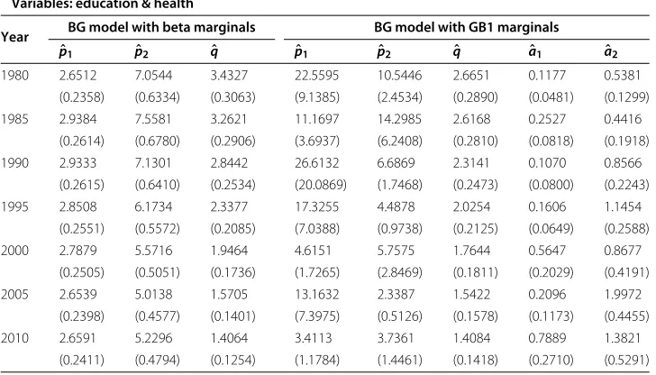
Table 1 Parameter estimates for the BG models (with beta and GB1 marginals) fitted to the variables education & health by maximum likelihood (standard errors in parenthesis)

Variables: education & health

Year BG model with beta marginals BG model with GB1 marginals

ˆ

p1 pˆ2 qˆ pˆ1 pˆ2 qˆ aˆ1 aˆ2

1980 2.6512 7.0544 3.4327 22.5595 10.5446 2.6651 0.1177 0.5381

(0.2358) (0.6334) (0.3063) (9.1385) (2.4534) (0.2890) (0.0481) (0.1299)

1985 2.9384 7.5581 3.2621 11.1697 14.2985 2.6168 0.2527 0.4416

(0.2614) (0.6780) (0.2906) (3.6937) (6.2408) (0.2810) (0.0818) (0.1918)

1990 2.9333 7.1301 2.8442 26.6132 6.6869 2.3141 0.1070 0.8566

(0.2615) (0.6410) (0.2534) (20.0869) (1.7468) (0.2473) (0.0800) (0.2243)

1995 2.8508 6.1734 2.3377 17.3255 4.4878 2.0254 0.1606 1.1454

(0.2551) (0.5572) (0.2085) (7.0388) (0.9738) (0.2125) (0.0649) (0.2588)

2000 2.7879 5.5716 1.9464 4.6151 5.7575 1.7644 0.5647 0.8677

(0.2505) (0.5051) (0.1736) (1.7265) (2.8469) (0.1811) (0.2029) (0.4191)

2005 2.6539 5.0138 1.5705 13.1632 2.3387 1.5422 0.2096 1.9972

(0.2398) (0.4577) (0.1401) (7.3975) (0.5126) (0.1578) (0.1173) (0.4455)

2010 2.6591 5.2296 1.4064 3.4113 3.7361 1.4084 0.7889 1.3821

(13)

Table 2 Parameter estimates for the BG models (with beta and GB1 marginals) fitted to the variables education & income by maximum likelihood (standard errors in parenthesis)

Variables: education & income

ˆ

1980 2.2431 3.3973 2.8809 2.1813 16.6110 2.6533 0.9603 0.2195

(0.2008) (0.3063) (0.2591) (0.5790) (13.5230) (0.2743) (0.2243) (0.1715)

1985 2.8775 3.7222 3.1934 4.3394 10.2173 2.7715 0.6321 0.3586

(0.2572) (0.3338) (0.2858) (1.4677) (5.6252) (0.2881) (0.1955) (0.1857)

1990 3.1691 3.6855 3.0715 6.4501 7.6217 2.6157 0.4702 0.4541

(0.2834) (0.3302) (0.2746) (2.7530) (3.5058) (0.2725) (0.1880) (0.1960)

1995 3.3196 3.3074 2.7070 6.3618 6.2069 2.3322 0.4907 0.4965

(0.2978) (0.2967) (0.2421) (2.4599) (2.2291) (0.2418) (0.1818) (0.1698)

2000 3.4652 3.0623 2.3826 5.8748 5.8042 2.0680 0.5420 0.4885

(0.3119) (0.2751) (0.2131) (2.2960) (2.0882) (0.2139) (0.2052) (0.1691)

2005 3.6366 2.8670 2.0777 7.2438 3.4311 1.8787 0.4773 0.7694

(0.3285) (0.2580) (0.1858) (3.2031) (0.8872) (0.1918) (0.2070) (0.1937)

2010 3.7596 2.7789 1.8944 3.4581 4.0863 1.8134 1.0309 0.6702

(0.3406) (0.2505) (0.1693) (1.0479) (1.1725) (0.1835) (0.3034) (0.1870)

the single-dimensional indices of the HDI, which are three normalized variables placed on scale 1-0. This structure of the data is specially representative in this case since we consider Beta and GB1 marginals for the BG models.

Income is represented by Gross National Income per capita measured in PPP 2005 US dollars, to make incomes comparable across countries and over time. The health com-ponent is represented by life expectancy at birth, which is considered an indicator of the health level.The education index is made up of two indicators, expected years of schooling and mean years of schooling, which are aggregated using the geometric mean. The first educational variable informs about the number of years that a child of school entrance

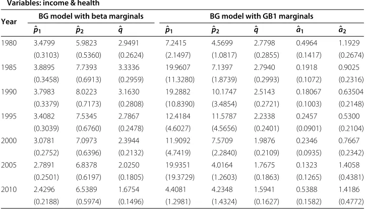
Table 3 Parameter estimates for the BG models (with beta and GB1 marginals) fitted to the variables income & health by maximum likelihood (standard errors in parenthesis)

Variables: income & health

ˆ

1980 3.4799 5.9823 2.9491 7.2415 4.5699 2.7798 0.4964 1.1929

(0.3103) (0.5360) (0.2624) (2.1497) (1.0817) (0.2855) (0.1417) (0.2674)

1985 3.8895 7.7393 3.3336 19.9607 7.1397 2.7940 0.1918 0.9025

(0.3458) (0.6913) (0.2959) (11.3280) (1.8739) (0.2993) (0.1072) (0.2316)

1990 3.7983 8.0223 3.1630 19.2882 10.1747 2.5143 0.18067 0.63504

(0.3379) (0.7173) (0.2808) (10.8390) (3.4854) (0.2721) (0.1003) (0.2148)

1995 3.4082 7.5345 2.7867 12.4184 11.5787 2.2338 0.2457 0.5300

(0.3039) (0.6760) (0.2478) (4.6027) (4.5656) (0.2401) (0.0901) (0.2104)

2000 3.0781 7.0973 2.3944 11.9092 7.5709 1.9876 0.2346 0.7667

(0.2752) (0.6396) (0.2132) (4.7419) (2.2840) (0.2109) (0.0935) (0.2342)

2005 2.7891 6.8378 2.0250 19.9351 4.0164 1.7675 0.1323 1.4058

(0.2501) (0.6197) (0.1805) (19.3729) (1.2603) (0.1863) (0.1265) (0.4381)

2010 2.4296 6.5389 1.6754 4.4081 4.2348 1.5941 0.5388 1.4186

(14)

Table 4 Parameter estimates for the BG model (BG truncated exponential marginals) fitted to the variables education & health by maximum likelihood (standard errors in

parenthesis)

Year Truncated exponential model

ˆ

p1 pˆ2 qˆ aˆ1 aˆ2

1980 3.4104 19.2541 1.3217 3.1388 4.1114

(0.3671) (4.0935) (0.2372) (0.4543) (0.6456)

1985 3.9159 17.3862 1.4386 2.7821 3.4638

(0.4287) (3.7250) (0.2519) (0.4325) (0.6248)

1990 4.1159 10.5428 1.6196 2.2094 2.1086

(0.4795) (2.0906) (0.2652) (0.4185) (0.5804)

1995 4.0476 6.7782 1.6363 1.7177 1.0854

(0.5304) (1.3450) (0.2499) (0.4271) (0.5825)

2000 3.8541 5.3537 1.5412 1.3568 0.5281

(0.5772) (1.1472) (0.2193) (0.4437) (0.6087)

2005 4.3824 3.8719 1.2821 1.6870 0.0000

(0.7229) (0.4862) (0.1420) (0.4704) (0.0427)

2010 3.9681 4.1826 1.1884 1.3861 0.0001

(0.7878) (1.0311) (0.1607) (0.5223) (0.6912)

age can expect to receive if prevailing patterns of age-specific enrollment rates persist throughout the child’s life (UNDP 2012). The second indicator reports the average num-ber of years of education received by people aged 25 and older, converted from education attainment levels using official durations of each level (Barro and Lee, 2013).

Originally, our sample comprised only 105 countries, covering less than the 75 percent of global population. We had non-available data for 26 countries for one or more years before 1995. In order to offer comparable results across periods and to not restricting the sample considerably, missing values have been estimated. The estimation of these missing

Table 5 Parameter estimates for the BG model (BG truncated exponential marginals) fitted to the variables education & income by maximum likelihood (standard errors in

parenthesis)

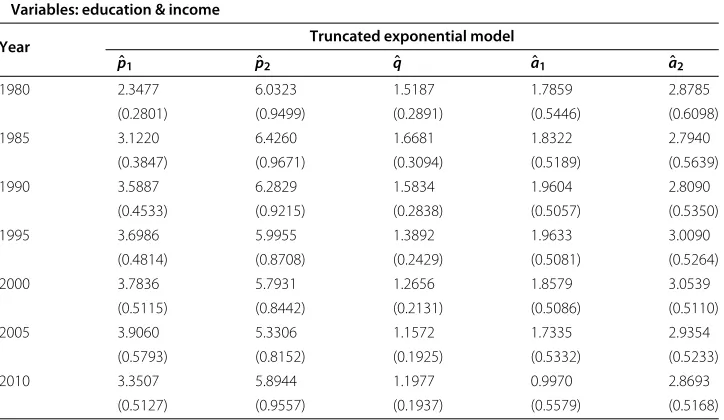
Variables: education & income

ˆ

1980 2.3477 6.0323 1.5187 1.7859 2.8785

(0.2801) (0.9499) (0.2891) (0.5446) (0.6098)

1985 3.1220 6.4260 1.6681 1.8322 2.7940

(0.3847) (0.9671) (0.3094) (0.5189) (0.5639)

1990 3.5887 6.2829 1.5834 1.9604 2.8090

(0.4533) (0.9215) (0.2838) (0.5057) (0.5350)

1995 3.6986 5.9955 1.3892 1.9633 3.0090

(0.4814) (0.8708) (0.2429) (0.5081) (0.5264)

2000 3.7836 5.7931 1.2656 1.8579 3.0539

(0.5115) (0.8442) (0.2131) (0.5086) (0.5110)

2005 3.9060 5.3306 1.1572 1.7335 2.9354

(0.5793) (0.8152) (0.1925) (0.5332) (0.5233)

2010 3.3507 5.8944 1.1977 0.9970 2.8693

(15)

Table 6 Parameter estimates for the BG model (BG truncated exponential marginals) fitted to the variables income & health by maximum likelihood (standard errors in parenthesis)

Variables: income & health

ˆ

1980 5.2910 5.6187 2.1441 1.7075 0.6332

(0.7765) (1.0281) (0.3450) (0.4689) (0.5700)

1985 6.0810 8.9083 2.0766 2.1172 1.3880

(0.7943) (1.6258) (0.3272) (0.4063) (0.5318)

1990 6.6056 9.9881 1.7975 2.5828 1.7600

(0.8013) (1.7123) (0.2787) (0.3801) (0.5043)

1995 6.6121 8.9254 1.5662 2.8884 1.7273

(0.8033) (1.4908) (0.2377) (0.3774) (0.4970)

2000 6.2010 7.4495 1.4527 2.8150 1.3495

(0.7880) (1.2753) (0.2108) (0.3768) (0.4997)

2005 6.5460 5.5399 1.3561 2.9102 0.6186

(0.9084) (0.9529) (0.1881) (0.3852) (0.5150)

2010 6.6966 4.1236 1.1760 3.1741 0.0000

(1.0480) (0.7957) (0.1720) (0.4275) (0.6583)

values has been based on two complementary methodologies which jointly offered feasi-ble and consistent results according to the sample: piecewise cubic Hermite interpolating polynomial (PCHI) and the average rate of change, which was used when PCHI offered unfeasible estimations or out of range results. The interpolated values have been obtained using the command pchip of the R package Signal, which uses the methodology described by Fritsch and Carlson (1980). After this procedure, our data set includes 132 countries whose indicators of income, health and education are available for eight points of time (see Appendix for details). Consequently, the sample covers over 90 percent of the world population during the whole period.

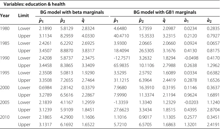
Table 7 Confidence intervals (95%) for the BG models (with beta and GB1 marginals) fitted to the variables education & health by maximum likelihood

Year Limit BG model with beta marginals BG model with GB1 marginals

ˆ

1980 Lower 2.1890 5.8129 2.8324 4.6480 5.7359 2.0987 0.0234 0.2835

Upper 3.1134 8.2959 4.0330 40.4710 15.3533 3.2315 0.2120 0.7927

1985 Lower 2.4261 6.2292 2.6925 3.9300 2.0665 2.0660 0.0924 0.0657

Upper 3.4507 8.8870 3.8317 18.4094 26.5305 3.1676 0.4130 0.8175 1990 Lower 2.4208 5.8737 2.3475 -12.7571 3.2632 1.8294 -0.0498 0.4170 Upper 3.4458 8.3865 3.3409 65.9835 10.1106 2.7988 0.2638 1.2962

1995 Lower 2.3508 5.0813 1.9290 3.5295 2.5792 1.6089 0.0334 0.6382

Upper 3.3508 7.2655 2.7464 31.1215 6.3964 2.4419 0.2878 1.6526

2000 Lower 0.6984 2.8142 0.3379 7.9680 16.3910 0.3195 0.1146 0.3637

Upper 3.2789 6.5616 2.2867 7.9990 11.3374 2.1194 0.9624 1.6891

2005 Lower 2.1839 4.1167 1.2959 -1.3359 1.3340 1.2329 -0.0203 1.1240

Upper 3.1239 5.9109 1.8451 27.6623 3.3434 1.8515 0.4395 2.8704

2010 Lower 2.1865 4.2900 1.1606 1.1016 0.9017 1.1305 0.2577 0.3451

(16)

Table 8 Confidence Intervals (95%) for the BG models (with beta and GB1 marginals) fitted to the variables education & income by maximum likelihood

ˆ

1980 Lower 1.8495 2.7970 2.3731 1.0465 -9.8941 2.1157 0.5207 -0.1166

Upper 2.6367 3.9976 3.3887 3.3161 43.1161 3.1909 1.3999 0.5556

1985 Lower 2.3734 3.0680 2.6332 1.4627 -0.8081 2.2068 0.2489 -0.0054

Upper 3.3816 4.3764 3.7536 7.2161 21.2427 3.3362 1.0153 0.7226

1990 Lower 2.6136 3.0383 2.5333 1.0542 0.7503 2.0816 0.1017 0.0699

Upper 3.7246 4.3327 3.6097 11.8460 14.4931 3.1498 0.8387 0.8383

1995 Lower 2.7359 2.7259 2.2325 1.5404 1.8379 1.8583 0.1344 0.1637

Upper 3.9033 3.8889 3.1815 11.1832 10.5759 2.8061 0.8470 0.8293 2000 Lower 1.0808 0.8424 0.5077 13.4885 12.1203 0.4423 0.1112 0.0826

Upper 4.0765 3.6015 2.8003 10.3750 9.8971 2.4872 0.9442 0.8199

2005 Lower 2.9927 2.3613 1.7135 0.9657 1.6922 1.5028 0.0716 0.3897

Upper 4.2805 3.3727 2.4419 13.5219 5.1700 2.2546 0.8830 1.1491

2010 Lower 3.0920 2.2879 1.5626 1.4042 2.5649 1.4537 0.4362 0.3037

Upper 4.4272 3.2699 2.2262 5.5120 7.1611 2.1731 1.6256 1.0367

4.2 Fitted models and results

The bivariate data consist of three pairs of variables (income,education), (income,health) and (education, health).

We have fitted the class of models given by Equation (4) with three specifications for the baseline CDFs:

• Fi(xi)=xi, with0≤xi≤1,i=1, 2(classical beta marginals), • Fi(xi)=xaii, with0≤xi≤1,ai>0,i=1, 2(GB1 marginals) and

• Fi(xi)= 1₁−₋exp_exp(−(−aaixi)i), with0≤xi≤1,ai>0,i=1, 2(BG truncated exponential

marginals).

Table 9 Confidence intervals (95%) for the BG models (with beta and GB1 marginals) fitted to the variables income & health by maximum likelihood

ˆ

1980 Lower 2.8717 4.9317 2.4348 3.0281 2.4498 2.2202 0.2187 0.6688

Upper 4.0881 7.0329 3.4634 11.4549 6.6900 3.3394 0.7741 1.7170

1985 Lower 3.2117 6.3844 2.7536 -2.2422 3.4669 2.2074 -0.0183 0.4486

Upper 4.5673 9.0942 3.9136 42.1636 10.8125 3.3806 0.4019 1.3564

1990 Lower 3.1360 6.6164 2.6126 -1.9562 3.3433 1.9810 -0.0159 0.2140

Upper 4.4606 9.4282 3.7134 40.5326 17.0061 3.0476 0.3773 1.0560

1995 Lower 2.8126 6.2095 2.3010 3.3971 2.6301 1.7632 0.0691 0.1176

Upper 4.0038 8.8595 3.2724 21.4397 20.5273 2.7044 0.4223 0.9424

2000 Lower 0.8471 4.5394 0.5105 56.4722 17.2919 0.4192 0.0219 0.1796

Upper 3.6175 8.3509 2.8123 21.2033 12.0475 2.4010 0.4179 1.2257 2005 Lower 2.2989 5.6232 1.6712 -18.0358 1.5462 1.4024 -0.1156 0.5471

Upper 3.2793 8.0524 2.3788 57.9060 6.4866 2.1326 0.3802 2.2645

2010 Lower 2.0008 5.3680 1.3822 1.8638 1.4273 1.2752 0.2287 0.4833

(17)

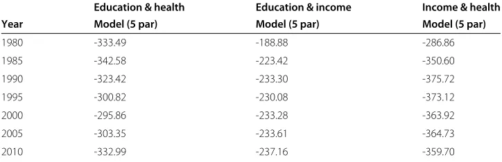
Table 10 AIC statistics obtained by maximum likelihood for the BG models with beta (3 parameters) and GB1 marginals (5 parameters) fitted to pairs of the variables: Education, Health and Income

Education & health Education & income Income & health

Year Model (3 par) Model (5 par) Model (3 par) Model (5 par) Model (3 par) Model (5 par)

1980 -292.88 -352.59 -174.12 -180.00 -279.48 -288.67

1985 -309.52 -354.03 -206.89 -217.35 -332.58 -354.54

1990 -304.40 -340.63 -213.99 -228.01 -344.03 -380.03

1995 -291.33 -313.41 -206.65 -217.94 -332.39 -370.94

2000 -291.77 -296.28 -207.64 -217.52 -325.00 -354.22

2005 -296.81 -306.00 -210.98 -213.52 -323.60 -340.72

2010 -330.82 -327.52 -215.63 -213.91 -317.16 -318.24

Smaller values indicate better fitted models.

The first model (with classical beta marginals) depends on 3 parameters, and the second and third models (with GB1 and BG truncated exponential marginals) are characterized by 5 parameters. The three models have been estimated by maximum likelihood using the equations given in Section 3.4. In total, we have fitted 7×3×3 = 63 different models. The initial estimates of the parameters have been obtained using Equations (17) to (19). In the case of the model with classical beta marginals, initial estimates are quite close to the ML estimators because they are based on sufficient statistics.

For the three pairs of variables, we have compared both models using the Akaike information criterion (AIC), defined by (Akaike 1974)

AIC= −2 logL+2d; (21)

where logL=

ˆ θ

is the log-likelihood of the model evaluated at the maximum likeli-hood estimates anddis the number of parameters. We chose the model with the smallest value ofAICstatistic.

Tables 1, 2, 3, 4, 5 and 6 show the parameter estimates and their standard errors for the three alternative models considered: BG distribution with classical beta marginals (3 parameter model p1,p2,q) and with GB1 and BG truncated exponential marginals

(5 parameter model p1,p2,q,a1,a2), which have been fitted to pairs of the variables:

Table 11 AIC statistics obtained by maximum likelihood for the BG model (BG truncated exponential maginals) with 5 parameters fitted to pairs of the variables: education, health and income

Education & health Education & income Income & health

Year Model (5 par) Model (5 par) Model (5 par)

1980 -333.49 -188.88 -286.86

1985 -342.58 -223.42 -350.60

1990 -323.42 -233.30 -375.72

1995 -300.82 -230.08 -373.12

2000 -295.86 -233.28 -363.92

2005 -303.35 -233.61 -364.73

2010 -332.99 -237.16 -359.70

(18)

Education, Health and Income. In particular, Tables 1 and 4 show the results obtained for Education & Health, Tables 2 and 5 show the corresponding results for Educa-tion & Income, and Tables 3 and 6 for Income & Health. The estimaEduca-tions have been performed by maximum likelihood, focusing on quinquennial periods from 1980 to 2010. It can be seen that, assuming the asymptotic normality of the maximum like-lihood estimates, most of the estimates are statistically significant at a 0.05 level of significance.

In order to illustrate the interval estimation of the parameters in Section 3.4, we have included the asymptotic confidence intervals at 95 percent for the models with beta and GB1 marginals (Tables 7, 8 and 9).

0.0 0.2 0.4 0.6 0.8 1.0 0.0

0.2 0.4 0.6 0.8 1.0

Education

Health

0.0 0.2 0.4 0.6 0.8 1.0 0.0

0.2 0.4 0.6 0.8 1.0

Education

Health

0.0 0.2 0.4 0.6 0.8 1.0 0.0

0.2 0.4 0.6 0.8 1.0

Education

Health

Year 1990

0.0 0.2 0.4 0.6 0.8 1.0 0.0

0.2 0.4 0.6 0.8 1.0

Education

Health

Year 1995

0.0 0.2 0.4 0.6 0.8 1.0 0.0

0.2 0.4 0.6 0.8 1.0

Education

Health

0.0 0.2 0.4 0.6 0.8 1.0 0.0

0.2 0.4 0.6 0.8 1.0

Education

Health

0.0 0.2 0.4 0.6 0.8 1.0 0.0

0.2 0.4 0.6 0.8 1.0

Education

Health

(19)

Tables 10 and 11 show the values of theAICstatistic (Equation (21)) obtained for both candidate models fitted to three pairs of variables: Education & Health, Education & Income and Income & Health. Our estimates point out that the values ofAICstatistic for the BG model with GB1 marginals are lower than those observed for the BG distribution with classical beta marginals, except in the case of Education & Health and Education & Income for the year 2010. For the Education & Health data the best model is the model with GB1 marginals (except in 2000). In the case of Education & Income data the model with BG truncated exponential marginals outperforms the other two models. Finally, for Income & Health data, the model with GB1 marginals outperforms the BG truncated

0.0 0.2 0.4 0.6 0.8 1.0 0.0

0.2 0.4 0.6 0.8 1.0

Education

Health

0.0 0.2 0.4 0.6 0.8 1.0 0.0

0.2 0.4 0.6 0.8 1.0

Education

Health

Year 1985

0.0 0.2 0.4 0.6 0.8 1.0 0.0

0.2 0.4 0.6 0.8 1.0

Education

Health

0.0 0.2 0.4 0.6 0.8 1.0 0.0

0.2 0.4 0.6 0.8 1.0

Education

Health

0.0 0.2 0.4 0.6 0.8 1.0 0.0

0.2 0.4 0.6 0.8 1.0

Education

Health

Year 2000

0.0 0.2 0.4 0.6 0.8 1.0 0.0

0.2 0.4 0.6 0.8 1.0

Education

Health

Year 2005

0.0 0.2 0.4 0.6 0.8 1.0 0.0

0.2 0.4 0.6 0.8 1.0

Education

Health

(20)

exponential marginals model in 1980, 1985 and 1995 while in the other four years the BG truncated exponential marginals is the model that provides the best fit. These results imply that, in general terms, the accuracy of the estimates is higher for the models with 5 parameters.

As an illustration, Figures 1, 2, 3, 4, 5 and 6 present the contour plots for the BG distri-butions with classical beta marginals and GB1 marginals fitted to the pairs of variables: Education & Health, Education & Income and Income & Health for every five years dur-ing the period 1980-2010. The shape of this graphics supports the existence of a positive correlation among the variables considered, thus pointing out the suitability of the first type of BG model. The contour plots also reveal that the proposed models represent the

0.0 0.2 0.4 0.6 0.8 1.0 0.0

0.2 0.4 0.6 0.8 1.0

Education

Income

0.0 0.2 0.4 0.6 0.8 1.0 0.0

0.2 0.4 0.6 0.8 1.0

Education

Income

Year

0.0 0.2 0.4 0.6 0.8 1.0 0.0

0.2 0.4 0.6 0.8 1.0

Education

Income

0.0 0.2 0.4 0.6 0.8 1.0 0.0

0.2 0.4 0.6 0.8 1.0

Education

Income

Year 1995

0.0 0.2 0.4 0.6 0.8 1.0 0.0

0.2 0.4 0.6 0.8 1.0

Education

Income

0.0 0.2 0.4 0.6 0.8 1.0 0.0

0.2 0.4 0.6 0.8 1.0

Education

Income

0.0 0.2 0.4 0.6 0.8 1.0 0.0

0.2 0.4 0.6 0.8 1.0

Education

Income

(21)

0.0 0.2 0.4 0.6 0.8 1.0 0.0

0.2 0.4 0.6 0.8 1.0

Education

Income

0.0 0.2 0.4 0.6 0.8 1.0 0.0

0.2 0.4 0.6 0.8 1.0

Education

Income

0.0 0.2 0.4 0.6 0.8 1.0 0.0

0.2 0.4 0.6 0.8 1.0

Education

Income

0.0 0.2 0.4 0.6 0.8 1.0 0.0

0.2 0.4 0.6 0.8 1.0

Education

Income

Year

0.0 0.2 0.4 0.6 0.8 1.0 0.0

0.2 0.4 0.6 0.8 1.0

Education

Income

Year 2000

0.0 0.2 0.4 0.6 0.8 1.0 0.0

0.2 0.4 0.6 0.8 1.0

Education

Income

Year 2005

0.0 0.2 0.4 0.6 0.8 1.0 0.0

0.2 0.4 0.6 0.8 1.0

Education

Income

Year 2010

Figure 4 Contour plots for the BG model with GB1 marginals fitted to the variables Education & Income.

geography of the bivariate data adequately, being more accurate in the case of the BG dis-tribution with GB1 marginals, as concluded from the results of the Akaike information criteria.

5 Conclusions

(22)

0.0 0.2 0.4 0.6 0.8 1.0 0.0

0.2 0.4 0.6 0.8 1.0

Income

Health

0.0 0.2 0.4 0.6 0.8 1.0 0.0

0.2 0.4 0.6 0.8 1.0

Income

Health

0.0 0.2 0.4 0.6 0.8 1.0 0.0

0.2 0.4 0.6 0.8 1.0

Income

Health

0.0 0.2 0.4 0.6 0.8 1.0 0.0

0.2 0.4 0.6 0.8 1.0

Income

Health

Year 1995

0.0 0.2 0.4 0.6 0.8 1.0 0.0

0.2 0.4 0.6 0.8 1.0

Income

Health

Year 2000

0.0 0.2 0.4 0.6 0.8 1.0 0.0

0.2 0.4 0.6 0.8 1.0

Income

Health

0.0 0.2 0.4 0.6 0.8 1.0 0.0

0.2 0.4 0.6 0.8 1.0

Income

Health

Year 2010

Figure 5 Contour plots for the BG model with beta marginals fitted to the variables Income & Health.

The main properties of these three classes have been studied. Three specific bivariate BG distributions have been obtained. Finally, an empirical application with well-being data has been presented.

(23)

0.0 0.2 0.4 0.6 0.8 1.0 0.0

0.2 0.4 0.6 0.8 1.0

Income

Health

0.0 0.2 0.4 0.6 0.8 1.0 0.0

0.2 0.4 0.6 0.8 1.0

Income

Health

0.0 0.2 0.4 0.6 0.8 1.0 0.0

0.2 0.4 0.6 0.8 1.0

Income

Health

0.0 0.2 0.4 0.6 0.8 1.0 0.0

0.2 0.4 0.6 0.8 1.0

Income

Health

Year 1995

0.0 0.2 0.4 0.6 0.8 1.0 0.0

0.2 0.4 0.6 0.8 1.0

Income

Health

Year 2000

0.0 0.2 0.4 0.6 0.8 1.0 0.0

0.2 0.4 0.6 0.8 1.0

Income

Health

0.0 0.2 0.4 0.6 0.8 1.0 0.0

0.2 0.4 0.6 0.8 1.0

Income

Health

Figure 6 Contour plots for the BG model with GB1 marginals fitted to the variables Income & Health.

Appendix

The joint PDF of the different classes of bivariate beta distribution

The joint PDF of the bivariate random variable in (3) is (see Libby and Novick (1982), Jones (2001) and Olkin and Liu (2003)),

f(z1,z2)=

za1−1

1 z

a2−1

2 (1−z1)a2+b−1(1−z2)a1+b−1

B(a1,a2,b) (1−z1z2)a1+a2+b

, 0<z1,z2<1 (22)

where B(a1,a2,b) = (a1)(a2)(b)/ (a1 + a2 + b) and the marginal

(24)

three-parametric exponential family, where sufficient statistics for(a1,a2,b) are given

by,

_n

i=1

y1i(1−y2i) 1−y1iy2i

, n

i=1

y2i(1−y1i) 1−y1iy2i

, n

i=1

(1−y1i) (1−y2i) 1−y1iy2i

.

Forn=1, the distributions of the sufficient statistics are: 1−Z1Z2

Z1(1−Z2) ∼B

2(a2+b,a1)+1,

1−Z1Z2

Z2(1−Z1) ∼B

2(a1+b,a2)+1,

and

1−Z1Z2

(1−Z1) (1−Z2) ∼B

2(a1+a2,b)+1,

whereB2(a,b)denotes beta distribution of the second kind. The log-moments of (22) are:

E

logZ1(1−Z2) 1−Z1Z2

= ψ (a1)−ψ (a1+a2+b),

E

logZ2(1−Z1) 1−Z1Z2

= ψ (a2)−ψ (a1+a2+b),

E

log(1−Z1) (1−Z2) 1−Z1Z2

= ψ (b)−ψ (a1+a2+b).

The joint PDF of the bivariate beta density (8) is givenby (see El-Bassiouny and Jones (2009)),

f(z1,z2)=k

za1−1

1 (1−z1)A−a1−1z2a2−1(1−z2)A−a2−1 (1−z1z2)A

× 2F1

A,a4;A−a2;

z1(1−z2)

1−z1z2

,

(23)

whereA=a1+a2+a3+a4,k−1=B(a1,a3)B(a2,a1+a3+a4)and 2F1[..; .; ] denote

the Gauss hypergeometric function.

The expression for thefV,W(v,w)function is given by (see Arnold and Ng 2011),

fV,W(v,w)=

∞

0

∞

0

(u4+u5)v

u4/(w−u5)

f(v,w,u3,u4,u5)du3du4du5, u,w>0, (24)

where

f(v,w,u3,u4,u5) =

(u3+u5) (u4+u5)

5

i=1 (ai)

[(v(u4+u5)−u3)]a1−1

×[w(u3+u5)−u4]a2−1 5

i=3

uai−1

i exp{−[u3w+u4v+u5(v+w+1)]},

whereu4/w−u5<u3< (u4+u5)v,u4,u5,v,w>0.

Description of the data set

The list of countries used in the analysis are the following: