Comparing Techniques for Estimating Flame Temperature of Prescribed Fires

(1)

Comparing Techniques for Estimating Flame Temperature of

Prescribed Fires

Deborah K. Kennard1, Kenneth W. Outcalt2, David Jones2, and Joseph J. O’Brien2

1

Southern Research Station USDA Forest Service

502 Devall Drive Auburn, AL 36849

2

Southern Research Station USDA Forest Service

320 Green Street Athens, GA 30602

ABSTRACT

A variety of techniques that estimate temperature and/or heat output during fires are available. We assessed the predictive ability of metal and tile pyrometers, calorimeters of different sizes, and fuel consumption to time-temperature metrics derived from thick and thin thermocouples at 140 points distributed over 9 management-scale burns in a longleaf pine forest in the southeastern US. While all of these devices underestimate maximum flame temperatures, we found several to be useful for characterizing other metrics of fire behavior. While the degree to which thermocouples underestimated maximum temperatures was based on thickness, metrics derived from thermocouple data that integrated time and temperature minimized this discrepancy between thin and thick thermocouples. Thermocouples also provided the most detailed spatial and temporal data of the devices tested. Pyrometers underestimated maximum temperatures relative to thermocouples, but due to their low cost, can be useful for examining spatial variation in temperature during fires. Use of calorimeters is disadvantageous given their lack of precision and high labor cost. Simple fire behavior observations taken during burns and indicators of fire severity observed post-burn were inexpensive to estimate and revealed useful differences among fires. Due to the wide variation among these techniques in cost, labor, accuracy, and level of detail of results, their suitability for a particular project will vary according to research objectives and available resources. Researchers should ensure that the fire behavior parameter measured has a logical relationship to the effect of interest, is measured at an appropriate level of detail, and is reported with attention to the limitations of the measuring devices used.

(2)

INTRODUCTION

Estimating flame temperature and duration has become increasingly common in studies of the ecological effects of fire. Researchers have found estimates of fire temperatures and their durations correlate well with fire effects on specific plant parts (seeds, roots, cambium) or soil components (e.g., Auld and O’Conner 1991, Dickinson and Johnson 2001). Time-temperature curves are most commonly measured using thermocouples deployed with data loggers. However due to the high cost of data loggers, researchers often rely on less expensive tools such as pyrometers or calorimeters to provide an index of flame temperature or heat release. Pyrometers, namely pellets, paints, or crayons manufactured to melt or change colors at specific temperatures, are commonly used to estimate fire temperatures in ecological studies (Fonteyn et al. 1984, Hobbs et al. 1984, Gibson et al. 1990, Cole et al. 1992, Franklin et al. 1997, Lippincott 2000, Menges and Deyrup 2001, Iverson et al. 2004). Calorimeters have been used to estimate heats of vaporization by measuring water mass lost from open containers exposed to fire (Beaufait 1966, Knight 1981, Moreno and Oechel 1989, Perez and Moreno 1998).

This suite of techniques commonly used by fire ecologists vary considerably in cost, level of detail of results, and most importantly accuracy. Notably, few of these instruments measure actual flame temperatures (or heat release in the case of calorimeters) as is sometimes erroneously reported in the ecological literature, but rather measure their own temperature during a fire (e.g. the device temperature), or their own heat gain in the case of calorimeters. While the device temperature is a function of the heat flux it receives

from the fire and therefore highly correlated with physical aspects of fire, it is also a function of the device’s heat budget (heat gained – heat lost). The accuracy of different devices in measuring flame temperatures (or heat release) will therefore vary considerably due to their different heat budgets, which is influenced by their size, color, and material construction. In most cases, these devices are sensitive to heating duration and therefore underestimate true maximum flame temperature. The data they provide represents more accurately an integration of flame temperature and duration. Yet this fact does not necessarily diminish their utility for characterizing useful fire behavior parameters. In many cases, parameters that integrate time and temperature are more useful for predicting ecological effects than maximum temperatures, since instantaneous maximum temperatures in forest fire flames should all attain the same value (approximately 1100 C; Martin et al. 1969) regardless of rate of spread, flame length, flame width, etc… (Van Wagner and Methven 1978).

Due to the variation among these techniques in accuracy, cost, level of detail in results, and the amount of labor required for deployment, their suitability for a particular project will vary depending on research objectives and available resources. Where resources do not allow sophisticated measuring tools, and research or management objectives do not require them, rather simple measuring devices may be used as practical alternatives. In order for fire ecologists or fire managers to choose the best possible tool to meet their needs, they must be aware of the advantages and drawbacks of the suite of tools available.

(3)

to a variety of metrics derived from time-temperature curves as measured by thermocouples (Perez and Moreno 1998, Wally et al., in press). Here, we extend these studies by comparing the predictive ability of two thicknesses of thermocouples, two types of pyrometers, and two sizes of calorimeters to the same time-temperature metrics as those used by Perez and Moreno (1998) and Wally et al. (in press). Because thermocouples, pyrometers, or calorimeters are either too expensive or too labor intensive to deploy in many management scenarios or landscape-level research projects, we also compare the time-temperature metrics to a simple field estimate of fuel consumption. Finally, we provide a cost and labor comparison of these techniques.

METHODS

Site description

This study was conducted in naturally regenerated longleaf pine (Pinus palustris) stands at the Solon Dixon Forestry Education Center (SDFEC) in the lower coastal plain of Alabama, USA. The SDFEC is intensively managed for both wood production and research purposes. Of the Center’s 2,144 ha, approximately 23% are upland and bottomland hardwoods, 40% upland mixed pine-hardwoods, 33% even-aged pine plantations, and 4% regenerating cutover areas. In addition to longleaf pine, overstories of the stands used in this study contained loblolly pine (Pinus taeda), southern red oak (Quercus falcata), post oak (Quercus stellata), laurel oak

(Quercus laurelfolia), and turkey oak

(Quercus laevis). Understories are

predominately shrubs (10-20% cover), with yaupon hollow (Ilex vomitoria), Vaccinium spp., and gallberry (Ilex

glabra) comprising the dominant shrub

species. Grasses (5-10% cover) include

Andropogon spp., Panicum spp.,

Dicanthelium spp., among others. All of

the stands used in this study were managed with early-growing season burns on a three-year rotation since the mid-1970s.

Average summer and winter temperatures at the SDFEC are 26o C and 9o C, respectively. Annual precipitation is 148 cm. Soils are deep and well-drained sandy loams that are strongly to very strongly acidic with low organic matter.

Sampling design

(4)

and the fire developed into a flanking then heading fire. The broader implications of how the four fuel reduction treatments in the FFS study affect actual fuel loads and reduce the risk of catastrophic wildfire, the primary objective of the FFS study, will be the focus of a separate paper. Our focus of this paper is the comparison of different techniques for estimating flame temperature.

At systematically arranged sampling points in each of these 9 plots we installed thermocouples, metal and ceramic tile pyrometers, calorimeters, and visually estimated preburn fuel loads and fuel consumption postburn. Methods used for each of these techniques are described below. Sampling intensity varied among the 9 burns (Table 1); additional sampling points consisting of only calorimeters and pyrometers were used in the burn-only and herbicide-and-burn plots so that spatial patterns of fire temperature could be examined for a separate study. In this study, we only focus on sampling points where thermocouples were deployed with calorimeters and pyrometers (140 sampling points).

For reasons explained in the introduction, we refer to the measurements as TC temperature (thermocouple temperature), MP temperature (metal pyrometer temperature), TP temperature (tile pyrometer temperature), and C heat uptake (heat uptake by calorimeters).

Thermocouples

We used HOBO® Type-K

Thermocouple loggers equipped with high temperature stainless-steel Type-K Thermocouple probes (Onset Computer Corporation, Cape Cod, MA, USA). The data loggers are easily buried due to their small dimensions (6 x 8 x 1.5 cm). They are battery powered and store data on a

microchip. Only thick thermocouple probes (4.8 mm diameter) were used for the 6 burns conducted in 2002. These probes consisted of a 304 stainless steel jacket packed with MgO, with an isolated Type K thermocouple junction at the tip. For 2 herbicide-and-burn plots burned in 2003, both thin (1 mm diameter) and thick diameter thermocouple probes were compared at a subset of points. At these points, the tips of the thin and thick probe thermocouples were positioned within 2 cm apart. At all points, loggers were placed in PVC tubes (8.8 cm wide, 13.2 cm long) with plastic caps on each end and buried below the soil surface. To prevent damage to loggers, litter and other available fuels were removed within ~50 cm of the point of burial. Thermocouple cables were buried in soil 5-10 cm deep between probes and loggers. Fuels within 1 m of the thermocouple probes were left in their natural state as far as was possible. Data loggers were programmed to record temperature every 2 seconds (4 plots) or 3 seconds (5 plots).

Tile Pyrometers

(5)

protected from rain with plastic bags; bags were removed the morning of burns.

Calorimeters and Metal Pyrometers

We used pint-sized (2002 burns) or half-pint sized (2003 burns) rectangular tin cans with screw caps (Yankee Containers, North Haven, CT, USA) for calorimeters. These particular cans were chosen because they were inexpensive (65-86 cents/ea.), had screw caps useful for transporting water, and would not melt at high temperatures unlike aluminum cans. We applied the same 14 different lacquers used for tile pyrometers around the top of each can (metal pyrometer). Calorimeters were wired to metal stakes at 30 cm height (opposite tile pyrometers) several days before burns and protected with plastic bags. On the day of burns, we removed plastic bags and put 50 ml of water in each can. After prescribed burns were completed, cans were capped, collected, and transported to the lab where remaining water was measured with a graduated cylinder or weighed. For each burn, 2-3 control calorimeters were placed in unburned areas to account for ambient evaporation. The amount of water vaporized from caloriometers during burns (accounting for ambient evaporation) was used to estimate heat uptake by cans as: heat uptake = [(80 cal/g water) x (g water)] +[(540 cal/g water) x (g water)], where 80 cal are needed to raise each gram of water from 20o C to boiling point and 540 cal are need to vaporize each gram of water (Beaufait 1966).

Fuel consumption estimates

Fuel loads were estimated within 3 weeks before burns in 1 m2 subplots centered on the sampling points. In each subplot, the percent cover and average

height of live trees/shrubs, dead trees/shrubs, vines, grasses, and forbs were estimated and used to calculate volumes. Biomass for these various fractions was then estimated using regression models derived from 150 1-m2 plots (located in the same treatment units) where the same method was used to estimate fuel volumes before fuels were destructively sampled and the dry masses determined: live tree/shrub (biomass g [ln+1] = 0.552 volume (cm3) + 0.104, r2 = 0.63), dead tree/shrub (biomass g [ln+1] = 0.462 volume (cm3) + 0.295, r2 = 0.52), vines (biomass g [ln+1] = 0.423 volume (cm3) + 0.515, r2 = 0.53), grasses (biomass g [ln+1] = 0.475 volume (cm3) + 0.360, r2 = 0.53), and forbs (biomass g [ln+1] = 0.420 volume (cm3) + 0.100, r2 = 0.54). Litter depth was measured in the center of the subplot. Litter mass was calculated from depth using a litter density of 0.039 g/cm3 derived from 900 1ft2 plots that were destructively sampled in the same treatment units. In a 1 m transect bisecting the subplot, the number of intercepts of fuels in four size classes (0-.6 cm, .6-2.5 cm, 2.5-7.6 cm, > 7.6 cm) were counted. Number of intercepts were used to calculate volumes and masses (assuming an overall density of 0.01 g/cm3) of these down woody fuels using Brown’s equations (Brown 1974). Immediately following fires, the percent burn of each subplot was visually estimated.

Statistical analysis

Following Perez and Moreno (1998) and Wally et al. (in press) we calculated six metrics of TC temperatures:

1. One-minute mean about the maximum (MEAN);

(6)

3. Time elapsed where instantaneous maximum > 60o C (TIME60);

4. Time elapsed where instantaneous maximum > 150o C (TIME150);

5. Integrated area under the instantaneous maximum curve over a threshold of 60o C (AREA60); and

6. Integrated area under the instantaneous maximum curve over a threshold of 150o C (AREA150).

As reported in Wally et al. (in press), the time elapsed during which the maximum temperature exceeds 150o C has been associated with calorimeter data (Perez and Moreno 1998), and the 60o C threshold corresponds to lethal temperature for plant cells (Alexandrov 1964).

We evaluated how closely pyrometers and calorimeters estimated the various metrics of TC temperatures by running linear regressions using each of the six metrics as response variables in separate analyses. We also evaluated which combinations of fuel components (standing fuel mass, down woody debris mass, litter mass), with or without pyrometer and calorimeter data, could predict TC temperatures by running forward multiple regressions in separate analyses using each of the thermocouple metrics. For each of these analyses, we use metrics derived from the thick thermocouples as the independent variable. Statistical analyses were performed using SPSS v. 9.0 (SPSS, Inc. 1998).

RESULTS

Summary statistics of weather conditions and standard descriptions of fire behavior are presented for each burn in Table 2. These simple observations show some variation among burns. For

example, the burns in Plots 2 and 10 were slower moving fires with higher residence times and shorter flames than the other 4 plots. The burns in plots 6 and 12, in contrast, were relatively faster moving fires, with higher flame lengths and wider flaming zones.

Thermocouples

Table 3 shows summary statistics of metrics calculated from thin and thick thermocouples. As shown in Figure 1, the increase in TC temperature to the maximum peak is slower in thick than in thin thermocouples due to the higher heat capacity of thick probes. Due to this slow response time, the maximum TC temperature is underestimated by thick thermocouples relative to the thinner thermocouples, particularly at high temperatures (Figure 2). These delayed responses are also reflected in the differences in TIME60 and TIME150 between the thick and thin thermocouples. Metrics that integrate time and temperature (MEAN, AREA60, and AREA150 ) were not as sensitive to delayed response times and therefore were very similar when measured by thick or thin thermocouples.

Pyrometers

(7)

underestimated MAX TC temperature by an average of 45o C and 14o C, respectively. In 2003, tile pyrometers underestimated MAX TC temperature by an average of 9o C, but metal pyrometers overestimated MAX TC temperature by an average of 51o C. If 2002 and 2003 burns are analyzed separately for metal pyrometers, adjusted R2 improve 3 to 18% (Table 4).

Calorimeters

Calorimeters were generally poor predictors of the thermocouple metrics, explaining only 12 to 36% of the variation in MEAN, MAX, TIME60, TIME150, AREA60, and AREA150 TC temperatures (Table 4, Figure 4). However, calorimeters did provide some information that pyrometers did not— the addition of calorimeter data to multiple regression models improved predictions of both MEAN and AREA60 TC temperatures. The size of cans used for calorimeters affected the amount of water vaporized- large cans tended to lose more water than small cans at points with similar thermocouple metrics. Information derived from control cans set out during each burn was not useful for accounting for ambient evaporation on a per sample basis. Approximately 25% of calorimeters showed no water loss or a water gain with the correction for ambient evaporation. This suggests small-scale variation in ambient evaporation complicates applying a single correction factor to many samples over a large area. As an example of this variation, the amount of water evaporated from control cans and cans retrieved from unburned points ranged from 6 to 22% (n = 23) of initial water content.

Fuel consumption indices

Pre-burn fuel load estimates were generally poor predictors of thermocouple metrics; only three (litter depth, intercepts of fuel > 7.6 cm diameter, calculated mass of down woody debris) were significant in multiple regression models (Table 5). Percent burn was more important in models predicting MEAN TC temperature than any of the fuel load estimates. The addition of metal pyrometers and calorimeters improved models, explaining 81% and 66% of the variation in MEAN and AREA60 TC temperatures, respectively.

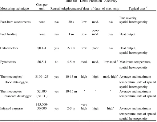
In Table 6, we summarize the estimated costs, times for deployment, levels of detail in data output, and appropriate uses of these different techniques. We also include, where applicable, a ranking of how closely these devices estimate instantaneous maximum temperatures.

DISCUSSION

(8)

and residence times (Stocks and Walker 1968, Gill and Knight 1991, Dickinson and Johnson 2001, Iverson et al. 2004). Considerably thinner thermocouples than those used in this study would be required to detect maximum temperatures and residence times more accurately. However, this necessarily creates a compromise between thermocouple wires that are sturdy enough to withstand field use but thin enough to register quick temperature changes. We found that using certain metrics that integrate time and temperature (e.g., MEAN, AREA60, AREA150) minimized these differences caused by thermocouple thickness. These metrics may prove more useful for predicting fire effects than instantaneous maximum temperature, since the duration of heat exposure is a significant variable determining cell death in plants and microbes, and the consumption of soil organic matter. The particular thick probes used in our study have also proved useful in estimating fireline intensity (Bova and Dickinson 2003). One noted advantage of using HOBO dataloggers is that their small size and relatively lower cost allowed us to sample extensively over the burn area, overcoming a common disadvantage of other datalogger types that restrict sampling to small areas (Wally et al. in press). Iverson et al. (2004) also noted this advantage of this particular datalogger type in their landscape-scale study of prescribed fires in oak-hickory forest.

Given their lower cost as compared to thermocouples, pyrometers predicted MEAN and MAX (as measured by the thick thermocouples) relatively well, explaining 60 to 82% of the variation of these metrics. The fact we used the thicker thermocouples as the reference for comparison in this study underestimates the degree of inaccuracy of pyrometers in

detecting maximum temperatures. We found tile pyrometers to be less accurate than metal pyrometers due to the insulating affect of the ceramic tiles. This insulating affect is particularly noticeable if the flame front approaches the tile pyrometer on the face opposite the painted surface. The water in our metal pyrometer/calorimeters absorbed heat creating an insulating affect as well, although this effect was less than that caused by the ceramic tiles. A significant drawback to the use of pyrometers is the inconsistent behavior of paints and the subjective interpretation of melted paints. Some paints melted poorly, even at temperatures above their designed melting point. Charring of the pyrometer surface made paints difficult to read. And, paints behaved differently on different material (e.g., soaked into porous ceramic, dripped on metal). These limitations, and the influence of pyrometer construction material, make comparison of pyrometer results across studies questionable.

(9)

different calorimeters across studies is also unreliable.

Pre-burn fuel load estimates were not useful for predicting thermocouple metrics. This was surprising considering the patchiness of fuels, particularly in the 3 plots that were thinned before burning. In contrast, a simple post-burn assessment of percent burn explained up to 36% of variation in thermocouple metrics. The predictive ability of this simple post-burn assessment of fuel consumption would likely be improved by including completeness of burn for different fuel components (litter/duff layer, woody debris, standing fuels), similar to commonly used post-burn severity classifications (Hungerford 1996). While not reliable for determining fire temperature, post-burn assessments may be suitable for assessing coarse-scale burn characteristics particularly over large areas and under limited budgets.

Due to the wide variation among these techniques in cost, labor, accuracy, and level of detail of results, their suitability for a particular project should depend on research objectives and available resources. Fire researchers and/or fire managers may rarely have the funds, labor, and time to choose the most accurate tool possible, but their objectives may not always require such accuracy. For example, physiological studies of fire damage to tree cambial tissue requires a different set of techniques than a study of the impact of fuel management on fire behavior over entire stands. Notably, the

simple fire behavior observations taken during the burns (flame height, rate of spread, residence time, etc…) revealed useful differences among the nine fires. While these techniques are easy, inexpensive to estimate, and can give adequate descriptions of management-scale burn impacts, we have noted that many fire research publications do not report these parameters. Minimally, studies should report these fire behavior parameters so that managers can replicate burns and their desired effects more easily or alter burn prescriptions to avoid undesirable outcomes. Where thermocouples, pyrometers, or calorimeters are used in fire research, authors should be careful to note the limitations of these devices when reporting results.

ACKNOWLEDGEMENTS

(10)

REFERENCES

Alexandrov, V.Y. 1964. Cytophysical and cytological investigations of heat resistance of plant cells toward the action of high and low temperature. Quarterly Review of Biology 39:35-77.

Auld, T.D., and M.A. O’Conner. 1991. Predicting patterns of post-fire germination in 35 eastern Australian Fabaceae. Australian Journal of Ecology. 16:53-70.

Beaufait, W.M. 1966. An integrating device for evaluating prescribed fires. Forest Science. 12:27-29.

Bova, A.S. and M.B. Dickinson. 2003. Making sense of fire temperatures: a thermocouple heat budget correlates temperatures and flame heat flux. In

Abstracts 88th Annual Meetings. The Ecological Society of America: Savanna

GA. 40-41.

Brown, J.K. 1974. Handbook for inventorying downed woody material. USDA Forest

Service Intermountain Forest and Range Experiment Station GTR INT-16. Ogden

UT 24 pp.

Cole, K.L., K.F. Klick, and N.B. Pavlovic. 1992. Fire monitoring during experimental burns at Indiana Dunes National Lakeshore. Natural Areas Journal. 12:177-183.

Dickinson, M.B., and E.A. Johnson. 2001. Fire Effects on Trees. In ‘Forest Fires:

Behavior and Ecological Effects.’ (Eds EA Johnson, K Miyanishi). Academic

Press: San Diego. 477-526.

Fonteyn, P.J., M.W. Stone, M.A. Yancy, and J.T.G. Baccus. 1984. Interspecific and intraspecific microhabitat temperature variations during a fire. American Midland Naturalist 112:246-250.

Franklin, S.B., P.A. Robertson, and J.S. Fralish. 1997. Small-scale fire temperature patterns in upland Quercus communities. Journal of Applied Ecology 34:613-630.

Gibson, D.J., D.C. Hartnett, and G.L.S. Merrill. 1990. Fire temperature heterogeneity in contrasting fire prone habitats: Kansas tallgrass prairie and Florida sandhill.

Bulletin of the Torrey Botanical Club, 117:349-356.

Gill, A.M., and I. Knight. 1991. Fire Measurement. In ‘Conference on Bushfire Modeling

and Fire Danger Rating systems.’ (Eds NP Cheney, AM Gill) (CSIRO Division

of Forestry, Yarralumla, ACT) 137-146.

(11)

Hungerford, R.D. 1996. Soils. Fire in Ecosystem Management Notes: Unit II-I. USDA Forest Service, National Advanced Resource Technology Center, Marana, Arizona.

Iverson, L.R., D.A Yaussy, J. Rebbeck, T.F. Hutchinson, R.P., Long, and A.M. Prasad. 2004. A comparison of thermocouples and temperature paints to monitor spatial and temporal characteristics of landscape-scale prescribed fires. International Journal of Wildland Fire. 13:1-12.

Knight, I.K. 1981. A simple calorimeter for measuring the intensity of rural fires.

Australian Forestry Research. 11:173-177.

Lippincott, C.L. 2000. Effects of Imperata cylindrica (L.) Beauv. (Cogongrass) invasion on fire regime in Florida sandhill. Natural Areas Journal. 20:140-149.

Martin, R.E., C.T. Cushwa, and R.L. Miller. 1969. Fire as a physical factor in wildland management. In ‘Proceedings of the Ninth Annual Tall Timbers Fire Ecology Conference.’ Tall Timbers Research Station, Tallahassee, FL. 271-288.

Menges, E.S., and M.A. Deyrup .2001. Postfire survival in south Florida slash pine: interacting effects of fire intensity, fire season, vegetation, burn size, and bark beetles. International Journal of Wildland Fire. 10:53-63.

Moreno, J.M., and W.C. Oechel. 1989. A simple method for estimating fire intensity after a burn in California chaparral. Acta Oecologia Planta. 10:57-68.

Perez, B., and J.M. Moreno. 1998. Methods for quantifying fire severity in shrubland-fires. Plant Ecology. 139:91-101.

SPSS, Inc., 1998. SPSS for Windows 9.0.0. SPSS Inc. Chicago, Illinois.

Stocks, B., and J. Walker. 1968. Thermocouple errors in forest fire research. Fire Technology 4:59-62.

Van Wagner, C.E., and I.R. Methven. 1978. Prescribed fire for site preparation in white and red pine. In ‘White and red pine symposium: Chalk River, ON, September 20-22, 1977.’ (Compiler DA Cameron) Symposium Proceedings O-P-6. Sault Ste. Marie, ON: Department of the Environment, Canadian Forestry Service, Great Lakes Forest Research Centre. 95-101.

(12)

Table 1. Number of thermocouple/datalogger pairs, pyrometers, and calorimeters used in each of 9 prescribed burns at a longleaf pine site in southern Alabama.

Thermocouples Pyrometers Calori-

Plot thick thin metal tile meters

burn

6 18 0 100 100 100

1 19 0 76 74 72

11 19 0 71 70 71

thin and burn

2 12 0 31 31 32

10 19 0 36 36 36

14 17 0 36 36 33

herbicide and burn

4 18 12 97 58 98

7 17 0 90 19 94

12 14 9 98 58 98

Total 153 21 635 482 634

Table 2. Weather conditions and standard fire behavior parameters observed during the 9

prescribed burns conducted in spring of 2002 and 2003 in southern Alabama.

Mean Mean Mean Mean

Total Max. Average Min. Direction/ Rate of Flame Fire Zone Residence burn time temp RH RH wind speed Spread Length Width Time Trt Unit Date (hrs) (C) (%) (%) (km/hr) (m/hr) (m) (m) (min)

burn only

6 4/17/2002 6 32 45.4 38 var / 8-10 62 1.1 .9 4.8

1 5/15/2002 12 29 30.0 25 NE / 5 63 .6 .4 3.1

11S 5/20/2002 7 25 31.0 27 NE / 5 37 .6 .6 4.0

11N 5/21/2002 9 26 28.8 26 N, NE / 5-13 47 .6 .4 3.9

thin and burn

2 4/5/2002 17 19 32.4 21 N, NE/10-23 27 .5 .5 8.3

14 5/1/2002 6 32 53.5 31 S,SW/15-23 45 .7 .8 3.8

10 5/22/2002 11 27 31.6 25 E / 8 27 .6 .5 5.1

herbicide and burn

4 4/15/2003 9 29 34.4 25.0 SE / 2-3 39 .7 .7 3.8

12 4/16/2003 10 29 38.1 29.0 S,SW / 3-5 57 1.6 .9 4.3

(13)

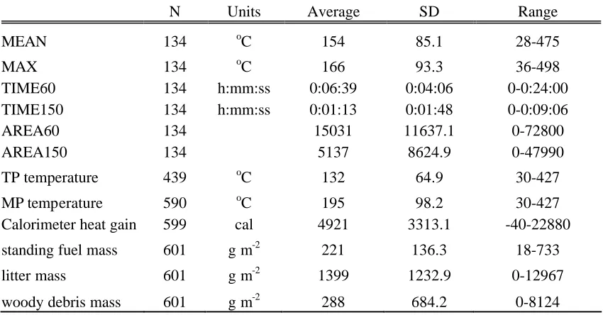
Table 3. Summary statistics of metrics derived from thermocouples, pyrometers, caloriometers, and fuel assessments. Only burned points, defined as more than half of the 1 m2 plot burned, are included in these statistics.

N Units Average SD Range

MEAN 134 oC 154 85.1 28-475

MAX 134 oC 166 93.3 36-498

TIME60 134 h:mm:ss 0:06:39 0:04:06 0-0:24:00

TIME150 134 h:mm:ss 0:01:13 0:01:48 0-0:09:06

AREA60 134 15031 11637.1 0-72800

AREA150 134 5137 8624.9 0-47990

TP temperature 439 oC 132 64.9 30-427

MP temperature 590 oC 195 98.2 30-427

Calorimeter heat gain 599 cal 4921 3313.1 -40-22880

standing fuel mass 601 g m-2 221 136.3 18-733

litter mass 601 g m-2 1399 1232.9 0-12967

woody debris mass 601 g m-2 288 684.2 0-8124

Table 4. Adjusted R2 values from linear regression analyses of metal

pyrometer temperature, tile pyrometer temperature, and caloriometer heat uptake on six metrices calculated from thick thermocouple data. For metal pyrometers, results are also analyzed separately for 2002 and 2003.

Thermocouple Metal pyrometers

metric Both years 2002 2003 Tile pyrometers Calorimeters

MEAN 0.68 0.81 0.79 0.62 0.34

MAX 0.68 0.82 0.79 0.61 0.34

TIME60 0.31 0.34 0.47 0.34 0.12

TIME150 0.52 0.61 0.58 0.46 0.32

AREA60 0.5 0.56 0.68 0.51 0.26

(14)

Table 5. Multiple regression results of fuel load estimates and percent burn on two thermocouple metrics (MEAN and AREA60) derived from thick thermocouples. Regressions were run both with and without pyrometer and caloriometer data in models.

Thermocouple

metric R2 Model

MEAN [ln] 0.31 percent burn

0.37 percent burn, litter depth [ln]

MEAN [ln] 0.71 max temperature (metal pyrometer)

0.76 max temperature (metal pyrometer), percent burn

0.79 max temperature (metal pyrometer), percent burn, calories (caloriometer) [ln] 0.79 max temperature (metal pyrometer), percent burn, calories (caloriometer) [ln],

litter litter depth [ln]

AREA60 0.12 litter depth

0.21 litter depth, percent burn

0.28 litter depth, percent burn, woody fuel > 3" diameter

AREA60 0.5 max temperature (metal pyrometer)

0.61 max temperature (metal pyrometer), calories (caloriometer)

0.66 max temperature (metal pyrometer), calories (caloriometer), woody mass

(15)

Table 6. Estimated cost, time for deployment, detail, precision, and accuracy of data, and typical uses of 7 techniques for estimating fire temperature, heat output, or fire severity. Infrared cameras, while not included in this study, are included here for comparison purposes.

Time for Detail Precision Accuracy

Measuring technique

Cost per

unit Reusable deployment of data of data of max temp Typical uses d

Post-burn assessments none n/a 30 s low mod. n/a

Fire severity, spatial heterogeneity

Fuel loading none n/a 1 m low

poor-mod. n/a Heat output

Calorimeters $0.1-1 yes 2-3 m low poor n/a Heat output,

spatial heterogeneity

Pyrometers $0.5-1 no 4-5 m mod. mod. low-mod.a Maximum temperature,

Thermocouples/ $100-125 yes 10-15 m high high mod.-highb Average and maximum

Hobo dataloggers temperature, rate of spread

spatial heterogeneity Thermocouples/ $2,500 yes 10-15 m " " " Average and maximum

Standard datalogger (36 TC) temperature, rate of spread

Infrared cameras

$15,000-50,000 yes 2-3 m

very

high high highc Average and maximum

temperature, rate of spread

a

Varies according to pyrometer material and subject to observer bias.

b

Depends on thermocouple thickness and type (shielded-aspirated thermocouples are most accurate in flames).

c

Only measures surface temperatures of objects, not flames. Accuracy dependent on knowing emissivity of objects and is affected by RH (including water vapor in smoke).

d

(16)

0 50 100 150 200 250 300 350 400 450 500

Time (hh:mm)

Temperature (C)

thin thermocouples thick thermocouples

15:30 16:00 16:30

Figure 1. Time x temperature curves for thin (0.1 cm diameter) and thick (0.48 cm

(17)

Mean temperature (C)

0 50 100 150 200 250 300 350 400

0 100 200 300 400

thick thermocouples

thin thermocouples

R2 = 0.9

Max temperature (C)

0 100 200 300 400 500 600

0 200 400 600

R2 = 0.76

Area > 60 C

0 10000 20000 30000 40000 50000 60000

R2 = 0.91

Time > 60 C

0 0.002 0.004 0.006 0.008 0.01 0.012

R2 = 0.61

Area > 150 C

0 5000 10000 15000 20000 25000 30000 35000 40000

0 10000 20000 30000 40000

R2_{= 0.96}

Time > 150 C

0 0.001 0.002 0.003

R2_{= 0.76}

Figure 2. Scatterplots and R2 values from regression analyses of six metrics derived from

(18)

A

0 100 200 300 400 500

MEAN temperature from logger (C)

Maximum pyrometer temperature

(C)

Can pyrometers

Tile pyrometers

0 100 200 300 400 500

MAX temperature from logger (C)

Maximum pyrometer temperature (C)

Can pyrometers

Tile pyrometers

B

Figure 3. Scatterplots of metal and tile pyrometer temperatures and: A. one-minute mean

about the maximum thermocouple temperature (MEAN) as measured by thick thermocouples, or B. instantaneous maximum temperature (MAX) as measured by thick thermocouples.

-5000 0 5000 10000 15000 20000 25000

0 100 200 300 400 500

MAX temperature from logger (C)

Net heat uptake of calorimeter (cal)

B

Figure 4. Scatterplots of net heat uptake of caloriometers and A. one-minute mean about

the maximum thermocouple temperature (MEAN) as measured by thick thermocouples, or B. instantaneous maximum temperature (MAX) as measured by thick thermocouples.

-5000 0 5000 10000 15000 20000 25000

0 100 200 300 400 500

MEAN temperature from logger (C)

Net heat uptake of calorimeter (cal)