R E S E A R C H Open Access
A survey of time consistency of dynamic risk
measures and dynamic performance measures in discrete
time: LM-measure perspective
Tomasz R. Bielecki · Igor Cialenco· Marcin Pitera
Received: 30 March 2016 / Accepted: 18 December 2016 /
© The Author(s). 2017Open AccessThis article is distributed under the terms of the Creative Commons Attribution 4.0 International License (http://creativecommons.org/licenses/by/4.0/), which permits unrestricted use, distribution, and reproduction in any medium, provided you give appropriate credit to the original author(s) and the source, provide a link to the Creative Commons license, and indicate if changes were made.
Abstract In this work we give a comprehensive overview of the time consistency property of dynamic risk and performance measures, focusing on a the discrete time setup. The two key operational concepts used throughout are the notion of the LM-measure and the notion of the update rule that, we believe, are the key tools for studying time consistency in a unified framework.
Keywords Time consistency·Update rule·Dynamic LM-measure·Dynamic risk
measure·Dynamic acceptability index·Measure of performance
MSC2010 91B30·62P05·97M30·91B06
“The dynamic consistency axiom turns out to be the heart of the matter.” A. Jobert and L. C. G. Rogers
Valuations and dynamic convex risk measures, Math Fin 18(1), 2008, 1–22.
Introduction
The goal of this work is to give a comprehensive overview of the time consistency property of dynamic risk and performance measures. We focus on discrete time setup, since most of the existing literature on this topic is dedicated to this case.
T. R. Bielecki ()·I. Cialenco
Department of Applied Mathematics, Illinois Institute of Technology, 10 W 32nd Str, Building E1, Room 208, Chicago, IL 60616, USA
e-mail: [email protected] I. Cialenco
e-mail: [email protected] M. Pitera
The time consistency surveyed in this paper is related to dynamic decision making subject to various uncertainties that evolve in time. Typically, decisions are made subject to the decision maker’s preferences, which may change in time and thus they need to be progressively assessed as an integral part of the decision making process. Naturally, the assessment of preferences should be done in such a way that the future preferences are assessed consistently with the present ones. This survey is focusing on this aspect of time consistency of a dynamic decision making process.
Traditionally, in finance and economics, the preferences are aimed at ordering cash and/or consumption streams. A convenient way to study preferences is to study them via numerical representations, such as (dynamic) risk measures, (dynamic) perfor-mance measures, or, more generally, dynamic LM-measures1(Bielecki et al. 2014a). Consequently, the study of the time consistency of preferences is also conveniently done in terms of their numerical representations. This work is meant to survey var-ious approaches to modelling and analysis of the time consistency of numerical representations of preferences.
As stated above, the objects of our survey—the dynamic LM-measures—are meant to “put a preference order” on the sets of underlying entities. There exists a vast literature on the subject of preference ordering, with various approaches towards establishing an order of choices, such as the decision theory or the expected util-ity theory, that trace their origins to the mid 20th century. We focus our attention, essentially, on the axiomatic approach to defining risk or performance measures.
The axiomatic approach to measuring risk of a financial position was initiated in the seminal paper by Artzner et al. (1999), and has been going through a flour-ishing development since then. The measures of risk introduced in (Artzner et al. 1999), called coherent risk measures, were meant to determine the regulatory capital requirement by providing a numerical representation of the riskiness of a portfolio of financial assets. In this framework, from mathematical point of view, the financial positions are understood as either discounted terminal values (payoffs) of portfolios, that are modeled in terms of random variables, or they are understood as discounted dividend processes, cumulative or bullet, that are modeled as stochastic processes. Although stochastic processes can be viewed as random variables (on appropriate spaces), and vice versa - random variables can be treated as particular cases of processes—it is convenient, and in some instances necessary, to treat these two cases separately—the road we are taking in this paper.
In the paper (Artzner et al. 1999), the authors considered the case of random variables, and the risk measurement was done at time zero only. This amounts to con-sidering a one period time model in the sense that the measurement is done today of the cash flow that is paid at some fixed future time (tomorrow). Accordingly, the related risk measures are referred to as static measures. Since then, two natural paths were followed: generalizing the notion of risk measure by relaxing or changing the set of axioms, or/and considering a dynamic setup. By dynamic setup we mean that the measurements are done throughout time and are adapted to the flow of available
information. In the dynamic setup, both discrete and continuous time evolutions have been studied, for both random variables and stochastic processes as the inputs. In the present work, we focus our attention on the discrete time setup, although we briefly review the literature devoted to continuous time.
This survey is organized as follows. We start with the literature review relevant to the dynamic risk and performance measures focusing on the time consistency prop-erty in the discrete time setup. In Section “Mathematical preliminaries”, we set the mathematical scene; in particular, we introduce the main notations used in this paper and the notion of LM-measures. Section “Approaches to time consistent assessment of preferences” is devoted to the time consistency property. There we discuss two generic approaches to time consistent assessment of preferences and point out sev-eral idiosyncratic approaches. We put forth in this section the notion of an update rule that, we believe, is the key tool for studying time consistency in a unified frame-work. Sections “Time consistency for random variables” and “Time consistency for stochastic processes” survey some concepts and results regarding time consistency in the case of random variables and in the case of stochastic processes, respectively. Our survey is illustrated by numerous examples that are presented in Section “Examples”. We end the survey with two appendices. In “Appendix” we provide a brief exposition of the three fundamental concepts used in the paper: the dynamic LM-measures, the conditional essential suprema/infima, and LM-extensions. Finally, in Appendix “Proofs” we collect proofs of several results stated throughout our survey.
Literature review
The aim of this section is to give a chronological survey of the developments of the theory of dynamic risk and performance measures. Although it is not an obvious task to establish the exact lineup, we tried our best to account for the most relevant works according to adequate chronological order.
We trace back the origins of the research regarding time consistency to Koopmans (1960) who put on the precise mathematical footing, in terms of the utility function, the notion of persistency over time of the structure of preferences.
Subsequently, in the seminal paper, Kreps and Porteus (1978) treat the time consis-tency at a general level by axiomatising the “choice behavior” of an agent by taking into account how choices at different times are related to each other; in the same work, the authors discuss the motivations for studying the dynamic aspect of choice theory.
Before we move on to reviewing the works on dynamic risk and performance measures, it is worth mentioning that the robust expected utility theory proposed by Gilboa and Schmeidler (1989) can be viewed as a more comprehensive theory than the one discussed in (Artzner et al. 1999); we refer to (Roorda et al. 2005) for the relevant discussion.
properties; c) provide particular examples of such functions. Each of the imposed axioms should have a meaningful financial or actuarial interpretation. For exam-ple, in (Artzner et al. 1999), a static coherent risk measure is defined as a function
ρ : L∞→ [−∞,∞]that is monotone decreasing (larger losses imply larger risk), cash-additive (the risk is reduced by the amount of cash added to the portfolio today), sub-additive (a diversified portfolio has a smaller risk) and positive homogenous (the risk of a rescaled portfolio is rescaled correspondingly), whereL∞ is the space of (essentially) bounded random variables on some probability space(,F,P)2. The descriptions or the representations of these functions, also called robust representa-tions, usually are derived via duality theory in convex analysis, and are necessary and sufficient in their nature. Traditionally, among such representations we find: representations in terms of the level or the acceptance sets; numerical representa-tions in terms of the dual pairings (e.g., expectarepresenta-tions). For example, the coherent risk measureρ mentioned above can be described in terms of its acceptance set Aρ = {X ∈ L∞|ρ(X)≤0}. As it turns out, the acceptance setAρ satisfies certain characteristic properties, and any setA with these properties generates a coherent risk measure via the representationρ(X)=inf{m∈R|m+X ∈A}. Alternatively, the functionρis a coherent risk measure if and only if there exists a nonempty setQ of probability measures, absolutely continuous with respect toP, such that
ρ(X)= − inf Q∈QE
Q[
X]. (1)
The setQ can be viewed as a set of generalized scenarios, and a coherent risk measure is equal to the worst expected loss under various scenarios. By relaxing the set of axioms, the static coherent risk measures were generalized to static convex risk measures and to an even more general class called monetary risk measures. See, for instance, (Szeg¨o 2002) for a survey of static risk measures, as well as (Cheridito and Li 2009, 2008). On the other hand, axiomatic theory of performance measures was originated in (Cherny and Madan 2009). A general theory of risk preferences and their robust representations, based on only two generic axioms, was studied in (Drapeau 2010, Drapeau and Kupper 2013).
Moving to the dynamic setup, we first introduce an underlying filtered probability space(,F,{Ft}t≥0,P), where the increasing collection ofσ-algebrasFt, t ≥0, models the flow of information that is accumulated through time.
Artzner et al. (2002b) and (Artzner et al. 2002a) study an extension of the static models examined in (Artzner et al. 1999) to the multiperiod case, assuming discrete time and discrete probability space. The authors proposed a method of constructing dynamic risk measures{ρt : L∞(FT)→ ¯L0(Ft), t =0,1. . . ,T}, by a backward recursion, starting withρT(X)= −X, and letting
ρt(X)= − inf Q∈QE
Q[−ρ
t+1(X)|Ft], 0≤t <T, (2)
where, as before,Qis a set of probability measures. If, additionally,Qsatisfies a property called recursivity or consistency (cf. (Riedel 2004)), namely
inf Q∈QE
Q[
Z |Ft]= inf Q∈QE
Q[ inf Q1∈Q
EQ1[Z|F
t+1]|Ft], t=0,1, . . . ,T−1,Z∈L∞, (3) then one can show that (2) is equivalent to
ρt(X)=ρt(−ρt+1(X)), 0≤t<T, X ∈L∞(FT). (4) The property (4) represents what has become known in the literature as thestrong time consistencyproperty. For example, ifQ= {P}, then the strong time consistency reduces to the tower property for conditional expectations. From a practical point of view, this property essentially means that assessment of risks propagates in a consis-tent way over time: assessing at timetfuture risk, represented by random variableX, is the same as assessing at timeta risky assessment ofXdone at timet+1 and repre-sented by−ρt+1(X).Additionally, the property (4) is closely related to the Bellman principle of optimality or to the dynamic programming principle (see, for instance, (Bellman and Dreyfus 1962; Carpentier et al. 2012).
Delbaen (2006) studies the recursivity property in terms ofm-stable sets of prob-ability measures, and also describes the time consistency of dynamic coherent risk measures in the context of martingale theory. The recursivity property is equivalent to properties known as time consistency and the rectangularity in the multi-prior Bayesian decision theory. Epstein and Schneider (2003) study time consistency and rectangularity property in the framework of “decision under ambiguity.”
It needs to be said that several authors refer to (Wang 2002) for an alternative axiomatic approach to time consistency of dynamic risk measures.
The first study of dynamic risk measures for stochastic processes (finite probabil-ity space and discrete time) is attributed to Riedel (2004), where the author introduced the (strong) time consistency as one of the axioms. Ifρt, t=0, . . . ,T,is a dynamic coherent risk measure, acting on the set of discounted terminal cash flows3, thenρis
strongly time consistentif the following implication holds true:
ρt+1(X)=ρt+1(Y) ⇒ ρt(X)=ρt(Y). (5) This means that if tomorrow we assess the riskiness ofXandYat the same level, then today X andY must have the same level of riskiness. It can be shown that for dynamic coherent risk measures, or more generally for dynamic monetary risk measures, property (5) is equivalent to (4).
Motivated by results regarding the pricing procedure in incomplete markets, based on use of risk measures, Roorda et al. (2005) study dynamic coherent risk measures (for the case of random variables on finite probability space and discrete time) and introduce the notion of (strong) time consistency; note that their work was similar and contemporaneous to (Riedel 2004). They show that strong time consistency entails recursive computation of the corresponding optimal hedging strategies. Moreover, time consistency is also described in terms of the collection of probability measures that satisfy the “product property,” similar to the rectangularity property mentioned above.
Similarly, as in the static case, the dynamic coherent risk measures were extended to dynamic convex risk measures by replacing sub-additivity and positive homogene-ity properties with convexhomogene-ity. In the continuous time setup, Rosazza Gianin (2002) links dynamic convex risk measures to nonlinear expectations org-expectations, and to Backward Stochastic Differential Equations (BSDEs). Strong time consistency plays a crucial role and, in view of (4), it is equivalent to the tower property for conditionalg-expectations. These results are further studied in a sequel of papers (Frittelli and Rosazza Gianin 2004; Peng 2004; Rosazza Gianin 2006), as well as in Coquet et al. (2002).
A representation similar to (1) holds true for dynamic convex risk measure
ρt(X)= − inf Q∈M(P)
EQ[X |Ft] +αtmin(Q)
, t =0,1, . . . ,T, (6)
whereM(P)is the set of all probability measures absolutely continuous with respect toP, and αmin is the minimal penalty function.4 The natural question of describ-ing (strong) time consistency in terms of properties of the minimal penalty functions was studied by Scandolo (2003). Also in (Scandolo 2003), the author discusses the importance in the dynamic setup of the special property called locality. It should be mentioned that locality property was part of the earlier developments in the the-ory of dynamic risk measures. For example, it was called dynamic relevance axiom in (Riedel 2004), and zero-one law in (Peng 2004). Similarly to previous studies, (Scandolo 2003) finds a relationship between time consistency, the recursive con-struction of dynamic risk measures, and the supermartingale property. These results are further investigated in Detlefsen and Scandolo (2005). Also in these works, it was shown that the dynamic entropic risk measure is a strongly time consistent convex risk measure.
Weber (2006) continues the study of dynamic convex risk measures for ran-dom variables in a discrete time setup and introduces weaker notions of time consistency acceptance and rejection time consistency. Mainly, the author stud-ies the law invariant risk measures, and characterizes time consistency in terms of the acceptance indicator at(X) = 1ρt(X)≤0 and in terms of the acceptance sets of the form Nt = {X | ρt(X) ≤ 0}. Along the same lines, F¨ollmer and Penner (2006) investigate the dynamic convex risk measures, representation of strong time consistency as a recursivity property, and they relate it to the Bellman principle of optimality. They also prove that the supermartingale prop-erty of the penalty function corresponds to the weak or acceptance/rejection time consistency. Moreover, the authors study the co-cycle property of the penalty func-tion for the dynamic convex risk measures that admit robust representafunc-tion (see Definition 50).
Artzner et al. (2007) continue to study the strong time consistency for dynamic risk measures, its equivalence with the stability property of test probabilities and with the optimality principle.
It is worth mentioning that Bion-Nadal (2004) studies dynamic monetary risk mea-sures in a continuous time setting and their time consistency property in the context of model uncertainty when the class of probability measures is not specified.
Motivated by optimization subject to risk criterion, Ruszczynski and Shapiro (2006a) elevate the concepts from (Ruszczy´nski and Shapiro 2006b) to the dynamic setting, with the main goal to establish conditions under which the dynamic programming principle holds.
Cheridito and Kupper (2011) introduce the notion of aggregators and generators for dynamic convex risk measures and give a thorough discussion about the com-position of time-consistent convex risk measures in the discrete time setup, for both random variables and stochastic processes. They link time consistency to one step dynamic penalty functions. In this regard, we also refer to (Cheridito et al. 2006; Cheridito and Kupper 2009).
Jobert and Rogers (2008) take the valuation concept as the starting point, rather than the dynamics of acceptance sets, with the valuation functional being the nega-tive of a risk measure. To quote the authors (strong) “time consistency is the heart of the matter.” Kloeppel and Schweizer (2007) use dynamic convex risk measures for valuation in incomplete markets, where the time consistency plays a key role. Cherny (2007) uses dynamic coherent risk measure for pricing and hedging European options; see also (Cherny and Madan 2006).
Roorda and Schumacher (2007) study the weak form of time consistency for dynamic convex risk measure.
Bion-Nadal (2006) continues to study various properties of dynamic risk mea-sures, both in discrete and in continuous time, mainly focusing on the composition property mentioned above, and thus on the strong time consistency. The composition property is characterized in terms of stability of probability sets. The author defines theco-cycle condition for the penalty functionand shows its equivalence to strong time consistency. In the followup paper, (Bion-Nadal 2008), the author continues to study the characterization of time consistency in terms of the co-cycle condition for minimal penalty function. For further related developments in the continuous time framework see (Bion-Nadal 2009b).
Observing that Value at Risk (V@R) is not strongly time consistent, Boda and Filar (2006), and Cheridito and Stadje (2009) construct a strongly time consistent alternative to V@R by using a recursive composition procedure.
Tutsch (2008) gives a different perspective on time consistency of convex risk measures by introducing the update rules5and generalizes the strong and weak form of time consistency via test sets.
The theory of dynamic risk measures finds its application in areas beyond the reg-ulatory capital requirements. For example, Cherny (2010) applies dynamic coherent risk measures to risk-reward optimization problems and in (Cherny 2009) to capi-tal allocation; Bion-Nadal (2009a) uses dynamic risk measures for time consistent pricing; Barrieu and El Karoui (2004; 2005; 2007) study optimal derivatives design under dynamic risk measures; Geman and Ohana (2008) explore the time consistency
in managing a commodity portfolio via dynamic risk measures; Zariphopoulou and Zitkovic (2010) investigate the maturity independent dynamic convex risk measures. In Delbaen et al. (2010), the authors establish a representation of the penalty func-tion of dynamic convex risk measure usingg-expectation and its relation to the strong time consistency.
There exists a significant literature on a special class of risk measures that sat-isfy the law invariance property. Kupper and Schachermayer (2009) prove that the only relevant, law invariant, strongly time consistent risk measure is the entropic risk measure.
For a fairly general study of dynamic convex risk measures and their time con-sistency we refer to (Bion-Nadal and Kervarec 2012) and (Bion-Nadal and Kervarec 2010). Acciaio et al. (2012) give a comprehensive study of various forms of time consistency for dynamic convex risk measures in a discrete time setup. This includes strong and weak time consistency, representations of time consistency in terms of acceptance sets, and the supermartingale property of the penalty function. We would like to point out the survey by Acciaio and Penner (2011) of discrete time dynamic convex risk measures. This work deals with (essentially bounded) random variables and examines most of the papers mentioned above from the perspective of the robust representation framework.
Although the connection between BSDEs and the dynamic convex risk measures in a continuous time setting had been established for some time, it appears that Stadje (2010) was the first author to create a theoretical framework for studying dynamic risk measures in discrete time via the Backward Stochastic Difference Equa-tions (BSEs). Due to the backward nature of BSEs, the strong time consistency of risk measures played a critical role in characterizing the dynamic convex risk mea-sures as solutions of BSEs. In a series of papers, Cohen and Elliott further studied the connection between dynamic risk measures and BSEs (Cohen and Elliott 2010, 2011; Elliott et al. 2015).
F¨ollmer and Penner (2011) developed the theory of dynamic monetary risk mea-sures under Knightian uncertainty, where the corresponding probability meamea-sures are not necessarily absolutely continuous with respect to the reference measure. See also Nutz and Soner (2012) for a study of dynamic risk measures under volatility uncertainty and their connection toG-expectations.
From a slightly different point of view, Ruszczynski (2010) studies Markov risk measures, that enjoy strong time consistency, in the framework of risk-averse pref-erences; see also (Shapiro 2009, 2011, 2012; Fan and Ruszczy´nski 2014). Some concepts from the theory of dynamic risk measures are adopted to the study of the dynamic programming for Markov decision processes.
In the recent paper, Mastrogiacomo and Rosazza Gianin (2015) provide several forms of time consistency for sub-additive dynamic risk measures and their dual representations.
We recall that the main objective of use of risk measures for financial applications is mapping the level of risk of a financial position to a regulatory monetary amount expressed in units of the relevant currency. Accordingly, the key property of any risk measure is cash-additivityρ(X−m)=ρ(X)+m. Clearly, one can think of the risk measures as generalizations of V@R.
A concept that is, in a sense, complementary to the concept of risk measures, is that of performance measures, which can be thought as generalizations of the well known Sharpe ratio. In similarity with the theory of risk measures, the development of the theory of performance measures followed an axiomatic approach. This was ini-tiated by Cherny and Madan (2009), where the authors introduced the (static) notion of the coherent acceptability index–a function onL∞with values inR+that is mono-tone, quasi-concave, and scale invariant. As a matter of fact, scale invariance is the key property of acceptability indices that distinguishes them from risk measures, and, typically, acceptability indices are not cash-additive. The dynamic version of coher-ent acceptability indices was introduced by Bielecki et al. (2014b), for the case of stochastic processes, finite probability space, and discrete time. From now on, we will use as synonyms the termsmeasures of performance,performance measures, andacceptability indices.
As it turns out, the time consistency for measures of performance is a delicate issue. None of the forms of time consistency, which had been coined for dynamic risk measures, are appropriate for dynamic performance measures. In (Bielecki et al. 2014b), the authors introduce a new form of time consistency that is suitable for dynamic coherent acceptability indices. Letαt, t = 0,1, . . . ,T, be a dynamic coherent acceptability index acting onL∞(i.e., discounted terminal cash flows). We say thatαis time consistent if the following implications hold true:
αt+1(X)≥mt ⇒ αt(X)≥mt,
αt+1(X)≤nt ⇒ αt(X)≤nt, (7)
where X ∈ L∞, and mt,nt are Ft-measurable random variables. Biagini and Bion-Nadal (2014) study dynamic performance measures in a fairly general setup that generalize the results of (Bielecki et al. 2014b). Later, using the theory of dynamic coherent acceptability indices developed in (Bielecki et al. 2014b), Bielecki et al. (2013) propose a pricing framework, called dynamic conic finance, for divi-dend paying securities in discrete time. The time consistency property was at the core of establishing the connection between dynamic conic finance and classical arbi-trage pricing theory. The static conic finance, that served as motivation for (Bielecki et al. 2013), was introduced in (Cherny and Madan 2010). Finally, in recent papers (Bielecki et al. 2015b, Rosazza Gianin and Sgarra 2013), the authors elevate the notion of dynamic coherent acceptability indices to the case of sub-scale invariant performance measures. For that, BSDEs are used in (Rosazza Gianin and Sgarra 2013) and BSEs are used in (Bielecki et al. 2015b).
Bion-Nadal 2016). Also in (Bielecki et al. 2016), the authors study the strong time consistency of quasi-concave maps via the concept of certainty equivalence; see also (Frittelli and Maggis 2010).
To our best knowledge, (Bielecki et al. 2014a) is the only paper that combines into a unified framework the time consistency for dynamic risk measures and dynamic performance measure. It uses the concept of update rules that serve as a vehicle for connecting preferences at different times. We take the update rules perspective as the main tool for surveying the existing forms of time consistency.
We conclude this literature review by listing works, which in our opinion, are most relevant to this survey (not all of which are mentioned above though).
Dynamic coherent risk measures
• random variables, strong time consistency: Artzner et al. 2002a, 2002b; Roorda 2005.
• stochastic processes, strong time consistency: Riedel 2004; Artzner et al. 2007.
Dynamic convex risk measures,
• random variables, strong time consistency: (discrete time) (Bion-Nadal 2006; Boda and Filar 2006; Cheridito and Stadje 2009; Detlefsen and Scandolo 2005; F¨ollmer and Penner 2006; Frittelli and Scandolo 2006; Geman and Ohana 2008; Ruszczy´nski and Shapiro 2006a; Scandolo 2003), (Acciaio and Penner 2011; Acciaio et al. 2012; Bielecki et al. 2014a; Bielecki et al. 2016; Bion-Nadal 2008; Cheridito and Kupper 2009; Cohen and Elliott 2010, 2011; Elliott et al. 2015; Fasen and Svejda 2012; Iancu et al. 2015; Kupper and Schachermayer 2009; Mastrogiacomo and Rosazza Gianin 2015; Roorda and Schumacher 2015; Stadje 2010);
(continuous time) (Barrieu and El Karoui 2004, 2007; Bion-Nadal 2006, 2008, 2009b; Bion-Nadal and Kervarec 2012; Delbaen 2012; Delbaen et al. 2010; Frittelli and Rosazza Gianin 2004; Jiang 2008; Kl¨oppel and Schweizer 2007; Nutz and Soner 2012; Penner and R´eveillac 2014; Rosazza Gianin 2002, 2006; Sircar and Sturm 2015).
• random variables, supermartingale time consistency: (Scandolo 2003; Detlefsen and Scandolo 2005).
• random variables, acceptance/rejection time consistency: (Acciaio et al. 2012; Bielecki et al. 2014a; F¨ollmer and Penner 2006; Roorda and Schumacher 2007, 2015; Tutsch 2008; Weber 2006).
• stochastic processes, strong and supermartingale time consistency: (discrete time) (Bielecki et al. 2014a; Scandolo 2003), (continuous time) (Jobert and Rogers 2008)
Dynamic monetary risk measures, strong time consistency:
Dynamic acceptability indices: (Bielecki et al. (2014b); Biagini and Bion-Nadal (2014); Bielecki et al. (2013); Rosazza Gianin and Sgarra (2013); Bielecki et al. (2016); Frittelli and Maggis (2014); Bielecki et al. (2014a); Bielecki et al. (2015b)).
Mathematical preliminaries
Let(,F,F = {Ft}t∈T,P)be a filtered probability space, withF0 = {,∅}, and T= {0,1, . . . ,T}, whereT ∈Nis a fixed and finite time horizon. We will also use the notationT = {0,1, . . . ,T−1}.
For G ⊆ F we denote by L0(,G,P) and L¯0(,G,P) the sets of all G -measurable random variables with values in(−∞,∞)and[−∞,∞], respectively. In addition, we use the notation Lp(G) := Lp(,G,P), Ltp := Lp(Ft), and Lp := LTp, for p ∈ {0,1,∞}; analogously we define L¯0t. We also use the nota-tionVp := {(Vt)t∈T : Vt ∈ L
p
t }, for p ∈ {0,1,∞}.6 Moreover, we useM(P)to denote the set of all probability measures on(,F)that are absolutely continuous with respect toP, and we setMt(P):= {Q∈M(P) : Q|Ft =P|Ft}.
Throughout this paper,Xrelates to either the space of random variablesLp, or the space of adapted processesVp. IfX =Lp, then the elementsX ∈Xare interpreted as discounted terminal cash flow. On the other hand, ifX =Vp, then the elements ofX are interpreted as discounted dividend processes. All concepts developed for X = Vpcan be easily adapted to the case of the cumulative discounted value pro-cesses. The case of random variables can be viewed as a particular case of stochastic processes by considering cash flow with only the terminal payoff, i.e., stochastic pro-cesses such thatV =(0, . . . ,0,VT). Nevertheless, we treat this case separately for transparency. In both cases, we consider the standard pointwise order, understood in the almost sure sense. In what follows, we also make use of the multiplication operator denoted as·t and defined by:
m·t V := (V0, . . . ,Vt−1,mVt,mVt+1, . . .),
m·t X := m X, (8)
forV ∈ (Vt)t∈T|Vt ∈L0t
, X ∈ L0,m ∈ L∞t , andt ∈ T. In order to ease the notation, if no confusion arises, we drop·t from the above product, and we simply writemVandmXinstead ofm·tV andm·t X, respectively. For anyt∈Twe set
1{t}:=
⎧ ⎨ ⎩
(0 ,0, . . . ,0 t
,1,0,0, . . . ,0),ifX =Vp,
1 ifX =Lp.
For anym∈ ¯L0
t, the valuem1{t}corresponds to a cash flow of sizemreceived at timet. We use this notation for the case of random variables to present more unified definitions (see Appendix “Dynamic LM-measures”).
Remark 1We note that the spaceVp, endowed with the multiplication ·t, does not define a proper L0–module (Filipovic et al. 2009; Vogelpoth 2009) (e.g., in general,0·t V = 0). However, in what follows, we will adopt some concepts from L0-module theory, which naturally fit into our study. We refer the reader to (Bielecki et al. 2015a, 2016) for a thorough discussion on this matter.
We use the convention∞−∞ = −∞+∞ = −∞and 0·±∞ =0. Note that the distributive law does not hold true in general:(−1)(∞ − ∞)= ∞ = −∞ + ∞ =
−∞.Fort ∈TandX ∈ ¯L0define the (generalized)Ft-conditional expectation ofX by
E[X|Ft] := E[X+|Ft] −E[X−|Ft],
whereX+=(X∨0)andX−=(−X ∨0). See Appendix “Conditional expectation and conditional essential supremum/infimum” for some relevant properties of the generalized expectation.
ForX ∈ ¯L0 andt ∈ T, we will denote by ess inftX the unique (up to a set of probability zero),Ft-measurable random variable, such that
ess inf
ω∈A X =ess infω∈A (ess inftX), (9) for any A ∈ Ft. We call this random variable theFt-conditional essential infimum of X. Similarly, we define ess supt(X) := −ess inft(−X), and we call it the Ft -conditional essential supremum of X. Again, see Appendix “Conditional expectation and conditional essential supremum/infimum” for more details and some elementary properties of conditional essential infimum and supremum.
The next definition introduces the main object of this work.
Definition 1A familyϕ = {ϕt}t∈T of mapsϕt : X → ¯L0t is a Dynamic LM-measure ifϕsatisfies
1) (Locality)1Aϕt(X)=1Aϕt(1A·t X); 2) (Monotonicity) X ≤Y ⇒ϕt(X)≤ϕt(Y);
for any t∈T, X,Y ∈X and A∈Ft.
It is well recognized that locality and monotonicity are two properties that must be satisfied by any reasonable dynamic measure of performance and/or measure of risk, and in fact are shared by most, if not all, of such measures studied in the lit-erature. The monotonicity property is natural for any numerical representation of an order between the elements ofX. The locality property (also referred to as regularity, or zero-one law, or relevance) essentially means that the values of the LM-measure restricted to a setA∈Fremain invariant with respect to the values of the arguments outside of the same set A ∈ F; in particular, the events that will not happen in the future do not affect the value of the measure today.
Similarly, any convex (or concave) map is also local (cf.(Detlefsen and Scandolo 2005)). It is also worth mentioning that locality is strongly related to time consis-tency. In fact, in some papers locality is considered as a part of the time consistency property discussed below (see e.g. (Detlefsen and Scandolo 2009)).
In this paper, we only consider dynamic LM-measuresϕ, such that
0∈ϕt[X], (10)
for anyt ∈T. We impose this (technical) assumption to ensure that the mapsϕt that we consider are not degenerate in the sense that they are not taking infinite values for allX ∈Xon some setAt ∈Ftof positive probability, for anyt ∈T; in the literature, sometimes such maps are referred to asproper(Kaina and R¨uschendorf 2009). If this is the case, then there exists a family{Yt}t∈T, whereYt ∈X, such thatϕt(Yt)∈ L0t for anyt ∈T, and so we can consider mapsϕ˜given byϕ˜t(·):=ϕt(·)−ϕt(Yt), that satisfy assumption (10) and preserve the same order as the mapsϕt do. Typically, in the risk measure framework, one assumes thatϕt(0) = 0, which implies (10). However, here we cannot assume thatϕt(0)=0, as we will also deal with dynamic performance measures for whichϕt(0)= ∞.
Finally, let us note that in the literature, traditionally the dynamic risk measures are monotone decreasing. On the other hand, the measures of performance are mono-tone increasing. In view of condition 2) in Definition 1, whenever our LM-measure corresponds to a dynamic risk measure, it needs to be understood as the negative of that risk measure. In such cases, in order to avoid confusion, we refer to the respec-tive LM-measure as todynamic (monetary) utility measurerather than as dynamic (monetary) risk measure. See Appendix “Dynamic LM-measures” for details.
Approaches to time consistent assessment of preferences
In this section, we present a brief survey of approaches to time consistent assessment of preferences, or to time consistency—for short, that were studied in the literature. As discussed in the Introduction, time consistency is studied via numerical represen-tations of preferences. Various numerical represenrepresen-tations will be surveyed below, and discussed in the context of dynamic LM-measures.
To streamline the presentation, we focus our attention on the case of random variables, that isX =Lp, forp∈ {0,1,∞}.7Usually, the risk measures and the per-formance measures are studied on spaces smaller thanL0, such asLp, p∈ [1,∞]. This is motivated by the aim to obtain so called robust representation of such mea-sures (see Appendix “Dynamic LM-meamea-sures”), since a certain topological structure is required for that (cf. Remark 13). On the other hand,time consistencyrefers only to consistency of measurements in time, where no particular topological structure is needed, and thus most of the results obtained here hold true forp=0.
In Section “Generic approaches”, we outline two generic approaches to time con-sistent assessment of preferences: an approach based on update rules and an approach based on benchmark families. These two approaches are generic in the sense that nearly all types of time consistency can be represented within these two approaches. On the contrary, the approaches outlined in Section “Idiosyncratic approaches” are specific. That is to say, those approaches are suited only for specific types of time consistency, specific classes of dynamic LM-measures, specific spaces, etc.
Generic approaches
In this section, we outline two concepts that underlie the generic approaches to time consistent assessment of preferences: the update rules and the benchmark families. It will be seen that different types of time consistency can be characterized in terms of these concepts.
Update rules
The approach to time consistency using update rules was developed in Bielecki et al. (2014a). An update rule is a tool that is applied to preference levels, and used for relating assessments of preferences done using a dynamic LM-measure at different times.
Definition 2A familyμ= {μt,s : t,s ∈ T,t <s}of mapsμt,s : ¯L0s → ¯L0t is called an update rule ifμsatisfies the following conditions:
1) (Locality)1Aμt,s(m)=1Aμt,s(1Am);
2) (Monotonicity) if m≥m, thenμt,s(m)≥μt,s(m);
for any s>t, A∈Ft, and m,m ∈ ¯L0s.
Next, we give a definition of time consistency in terms of update rules.
Definition 3Letμbe an update rule. We say that the dynamic LM-measureϕ is
μ-acceptance (resp.μ-rejection) time consistent if
ϕs(X)≥ms (resp.≤) =⇒ ϕt(X)≥μt,s(ms) (resp.≤), (11)
for all s>t, s,t ∈T, X∈X, and ms ∈ ¯L0s. If property (11) is satisfied for s=t+1, t∈T, then we say thatϕis one-stepμ-acceptance (resp. one-stepμ-rejection) time consistent.
We see thatms andμt,s(ms)serve as benchmarks to which the measurements of
ϕs(X)andϕt(X)are compared, respectively. Thus, the interpretation of acceptance time consistency is straightforward: ifX ∈X is accepted at some future times∈T, at least at levelms, then today, at timet ∈T, it is accepted at least at levelμt,s(ms). Similar reasoning holds for the rejection time consistency. Essentially, the update rule
We started our survey of time consistency with Definition 3 since, as we will demonstrate below, this concept of time consistency covers various cases of time consistency for risk and performance measures that can be found in the existing lit-erature. In particular, it allows to establish important connections between different types of time consistency. The time consistency property of an LM-measure, in gen-eral, depends on the choice of the updated rule; we refer to Section “Time consistency for random variables” for an in-depth discussion.
It is useful to observe that the time consistency property given in terms of update rules can be equivalently formulated as a version of the dynamic programming principle (see (Bielecki et al. 2014a), Proposition 3.6): ϕ is μ-acceptance (resp.
μ-rejection) time consistent if and only if
ϕt(X)≥μt,s(ϕs(X)) (resp.≤), (12)
for any X ∈ X and s,t ∈ T, such that s > t. The interpretation of (12) is as follows: if the numerical assessment of preferences about X is given in terms of a dynamic LM-measure ϕ, then this measure is μ-acceptance time consistent if and only if the numerical assessment of preferences aboutX done at time t is greater than the value of the measurement done at any future time s > t and updated at timetviaμt,s. The analogous interpretation applies to the ejection time consistency.
Next, we define two interesting and important classes of update rules.
Definition 4Letμbe an update rule. We say thatμis
1) s-invariant, if there exists a family{μt}t∈Tof maps μt : ¯L0 → ¯L0t, such that
μt,s(ms)=μt(ms)for any s,t ∈T, s >t, and ms ∈ ¯L0s;
2) projective, if it is s-invariant andμt(mt)=mt, for any t∈T, and mt ∈ ¯L0t.
Remark 3If an update ruleμis s-invariant, then it is enough to consider only the corresponding family{μt}t∈T. Hence, with slight abuse of notation, we write
μ= {μt}t∈Tand call it an update rule as well.
Example 1The familiesμ1= {μ1t}t∈Tandμ2= {μ2t}t∈Tgiven by
μ1
t(m)=E[m|Ft], and μ2t(m)=ess inftm, m∈ ¯L0,
are projective update rules. It will be shown in Example5that there is a dynamic LM-measure that isμ2–time consistent but notμ1–time consistent.
Benchmark families
Definition 5
(i) A familyY= {Yt}t∈Tof setsYt ⊆X is a benchmark family if
0∈Yt and Yt+R=Yt,
for any t∈T.
(ii) A dynamic LM-measureϕis acceptance (resp. rejection) time consistent with respect to the benchmark familyY, if
ϕs(X)≥ϕs(Y) (r esp.≤) =⇒ ϕt(X)≥ϕt(Y) (r esp.≤), (13)
for all s≥t, X ∈X, and Y ∈Ys.
Informally, the “degree” of time consistency with respect toYis measured by the size ofY. Thus, the larger the setsYs are, for eachs∈T, the stronger the degree of time consistency ofϕ.
Example 2The families of setsY1= {Yt1}t∈TandY2= {Yt2}t∈Tgiven by
Y1
t =R and Yt2=X,
are benchmark families. They relate to weak and strong types of time consistency, as will be discussed later on.
For future reference, we recall from (Bielecki et al. 2014a, Proof of Proposition 3.9) thatϕ is acceptance (resp. rejection) time consistent with respect toY, if and only ifϕis acceptance (resp. rejection) time consistent with respect to the benchmark familyYgiven by
Yt := {Y ∈X :Y =1AY1+1AcY2,for someY1,Y2∈Yt andA∈Ft}. (14)
Relation between update rule approach and the benchmark approach
The difference between the update rule approach and the benchmark family approach is that the preference levels are chosen differently. Specifically, in the former approach, the preference level at timesis chosen as anyms ∈ ¯L0s, and then updated to the preference level at timet, using an update rule. In the latter approach, the pref-erence levels at both timessandtare taken asϕs(Y)andϕt(Y), respectively, for any reference objectY ∈Ys, whereYs is an element of the benchmark familyY.
These two approaches are strongly related to each other. Indeed, for any LM-measureϕand for any benchmark familyY, one can construct an update ruleμsuch thatϕis time consistent with respect toYif and only if it isμ-time consistent.
For example, in case of acceptance time consistency ofϕwith respect toY, using the locality ofϕ, it is easy to note that (13) is equivalent to
ϕt(X)≥ess sup A∈Ft
1A ess sup Y∈YA−,s(ϕs(X))
ϕt(Y)+1Ac(−∞)
whereY−A,s(ms) := {Y ∈ Ys : 1Ams ≥ 1Aϕs(Y)}andY= {Ys}s∈Tis defined in (14). Consequently, setting
μt,s(ms):=ess sup A∈Ft
1A ess sup Y∈Y−A,s(ms)
ϕt(Y)+1Ac(−∞)
,
and using (12), we deduce thatϕ satisfies (13) if and only ifϕ is time consistent with respect to the update ruleμt,s (see (Bielecki et al. 2014a, Proposition 3.9) for details). The analogous argument works for rejection time consistency.
Generally speaking, the converse implication does not hold true; the notion of time consistency given in terms of update rules is more general. For example, time consistency of a dynamic coherent acceptability index cannot be expressed in terms of a single benchmark family.
Idiosyncratic approaches
Each such approach to time consistency of a given LM-measure exploits the idiosyn-cratic properties of this LM-measure, which are not necessarily shared by other LM measures, and typically is suited only for a specific subclass of dynamic LM-measures. For example, in case of dynamic convex or monetary risk measures the time consistency can be characterized in terms of the relevant properties of associated acceptance sets and/or the dynamics of the penalty functions and/or the rectangular property of the families of probability measures. These idiosyncratic approaches, and the relevant references, were mentioned and briefly discussed in Section “Literature review”. Detailed analysis of each of these approaches is beyond the scope of this survey.
Time consistency for random variables
In this section, we survey the time consistency of LM-measures applied to ran-dom variables. Accordingly, we assume thatX = Lp, for a fixed p ∈ {0,1,∞}. We proceed with the discussion of various related types of time consistency, with-out much reference to the existing literature. Such references are provided in Section “Literature review”.
Weak time consistency
Definition 6A dynamic LM-measure ϕ is weakly acceptance (resp. weakly rejection) time consistent if
ϕt(X)≥ess inftϕs(X), (r esp. ϕt(X)≤ess suptϕs(X) ) for any X∈ Lpand s,t ∈T, such that s >t.
Propositions 1 and 2 provide some characterizations of weak acceptance time consistency.
Proposition 1Letϕ be a dynamic LM-measure on Lp. The following properties are equivalent:
1) ϕis weakly acceptance time consistent.
2) ϕisμ-acceptance time consistent, whereμis a projective update rule, given by
μt(m)=ess inftm. 3) The following inequality is satisfied
ϕt(X)≥ ess inf Q∈Mt(P)
EQ[ϕs(X)|Ft], (15)
for any X ∈Lp, s,t ∈T, s >t.
4) For any X ∈ Lp, s,t∈T, s>t, and mt ∈ ¯L0t, it holds that
ϕs(X)≥mt ⇒ϕt(X)≥mt. Similar results hold true for weak rejection time consistency.
For the proof of the equivalence between 1), 2), and 4), see (Bielecki et al. 2014a, Proposition 4.3). Regarding 3), note that any measureQ∈Mt(P)may be expressed in terms of a Radon-Nikodym derivative with respect to measureP.In other words, instead of (26), we may write
ϕt(X)≥ess inf Z∈Pt
E[Zϕs(X)|Ft],
wherePt := {Z ∈ L1 | Z ≥ 0, E[Z|Ft] = 1}. Thus, one can show equivalence between 1) and 3) noting that for anym ∈ ¯L0 we get ess inf
tm = ess infZ∈Pt E[Z m|Ft]. See (Bielecki et al. 2014a, Proposition 4.4) for the proof.
It is worth mentioning that Property 4) in Proposition 1 was suggested as the notion of (weak) acceptance and (weak) rejection time consistency in the context of scale invariant measures, called acceptability indices (cf. (Biagini and Bion-Nadal 2014; Bielecki et al. 2014b)).
Usually, the weak time consistency is considered for dynamic monetary risk mea-sures onL∞(cf. (Acciaio and Penner 2011) and references therein). This case lends itself to even more characterizations of this property.
Proposition 2Letϕ be a representable dynamic monetary utility measure8 on L∞. The following properties are equivalent:
1) ϕis weakly acceptance time consistent.
2) ϕis acceptance time consistent with respect to{Yt}t∈T, whereYt =R. 3) For any X ∈ Lpand s,t ∈T, s >t,
ϕs(X)≥0⇒ϕt(X)≥0. (16)
4) At+1⊆At, for any t ∈T, such that t<T . 5) For any Q∈M(P)and t ∈T, such that t<T ,
αmin
t (Q)≥EQ[αtmin+1(Q)|Ft],
whereαminis the minimal penalty function in the robust representation ofϕ.
Analogous results are obtained for weak rejection time consistency.
We note that equivalence of properties 1), 2), and 3) also holds true in the case ofX = L0, and not only for representable, but for any dynamic monetary utility measure; for the proof, see (Bielecki et al. 2014a, Proposition 4.3). Property 4) is a characterisation of weak time consistency in terms of acceptance sets, and property 5) gives a characterisation in terms of the supermartingale property of the penalty func-tion. For the proof of the equivalence of 3), 4), and 5), see (Acciaio and Penner 2011, Proposition 33).
The next result shows that weak time consistency is indeed one of the weakest forms of time consistency, in the sense that the weak time consistency is implied by any time consistency generated by a projective update rule; we refer to (Bielecki et al. 2014a, Proposition 4.5) for the proof.
Proposition 3Letϕbe a dynamic LM-measure on Lp, and letμbe a projective update rule. Ifϕisμ-acceptance (resp.μ-rejection) time consistent, thenϕis weakly acceptance (resp. weakly rejection) time consistent.
Remark 4An important feature of the weak time consistency is its invariance with respect to monotone transformations. Specifically, let g : ¯R → ¯R be a strictly increasing function and letϕ be a weakly acceptance/rejection time consis-tent dynamic LM-measure. Then,{g◦ϕt}t∈Tis also a weakly acceptance/rejection time consistent dynamic LM-measure.
Remark 5In the case of general LM-measures, the weak time consistency may
not be characterized as in 2) of Proposition2. For example, ifϕ is a (normalized) acceptability index, thenϕt(R)= {0,∞}, for t ∈T, which does not agree with 4) in Proposition1.
Strong time consistency
It is fair to mention, that this form of time consistency also appears in the insur-ance literature, as the iterative property, and it is related to the mean value principle (Gerber 1974; Goovaerts and De Vylder 1979).
We start with the definition of strong time consistency.
Definition 7Letϕbe a dynamic LM-measure on Lp. Then,ϕis said to be strongly time consistent if
ϕs(X)=ϕs(Y) =⇒ ϕt(X)=ϕt(Y), (17) for any X,Y ∈Lpand s,t∈T, such that s>t.
Strong time consistency gains its popularity and importance due to its equiv-alence to the dynamic programming principle. This equivequiv-alence, as well as other characterisations of strong time consistency, are the subject of the following two propositions.
Proposition 4Letϕ be a dynamic LM-measure on Lp. The following properties are equivalent:
1) ϕis strongly time consistent.
2) There exists an update ruleμsuch thatϕis bothμ-acceptance andμ-rejection time consistent.
3) ϕis acceptance time consistent with respect to{Yt}t∈T, whereYt =Lp. 4) There exists an update ruleμsuch that for any X ∈Lp, s,t ∈T, s>t,
μt,s(ϕs(X))=ϕt(X). (18) 5) There exists a one-step update ruleμsuch that for any X ∈Lp, t∈T, t<T ,
μt,t+1(ϕt+1(X))=ϕt(X).
See Appendix “Proofs” for the proof of Proposition 4. Property 4) in this propo-sition is referred to as Bellman’s principle or the dynamic programming principle. Also, note that 5) implies that any strongly time consistent dynamic LM-measure can be constructed using a backward recursion starting fromϕT := , where is an LM-measure. See (Cheridito and Kupper 2011) where the recursive construction for dynamic risk measures is discussed in details.
An important, and frequently studied, type of strong time consistency is the strong time consistency for dynamic monetary risk measures on L∞(cf. (Acciaio and Penner 2011) and references therein). As the next result shows, there are more equivalences that are valid in this case.
Proposition 5Letϕbe a representable dynamic monetary utility measure on L∞. The following properties are equivalent:
1) ϕis strongly time consistent.
2) ϕis recursive, i.e., for any X∈ Lp, s,t ∈T, s >t,
3) At =At,s+As, for all t,s∈T, s >t. 4) For any Q∈M(P), t,s∈T, s >t,
αmin
t (Q)=αmint,s (Q)+EQ[αmins (Q)|Ft].
5) For any X ∈ Lp, Q ∈M(P), s,t ∈T, s>t,
ϕt(X)−αmint (Q)≤ EQ[ϕs(X)−αsmin(Q)|Ft].
For the proof see, for instance, (Acciaio and Penner 2011, Proposition 14).
Remark 6 (i) In general, for dynamic LM-measures, the strong time consistency does not imply either the weak acceptance or weak rejection time consistency. Indeed, let us considerϕ= {ϕt}t∈T, such thatϕt(X)=t (resp.ϕt(X)= −t) for all X ∈ L0. Sinceϕt(0)=t ≥ess inftϕs(0)=s (resp.−t ≤ −s), for s>t, we conclude thatϕis not weakly acceptance (resp. weakly rejection) time consistent. However, since ϕt(X) = ϕt(ϕs(X)) for any X ∈ L0, then ϕ is strongly time consistent. We note, that if the update rule in Definition 7 is projective, as it is usually the case for dynamic monetary risk measures, then, due to Proposition 3, the strong time consistency implies the weak time consistency.
(ii) It is worth mentioning that, in principle, strong time consistency is not suited for acceptability indices (Bielecki et al. 2014b, 2015b; Cherny and Madan 2009). Letϕ be a scale invariant dynamic LM-measure, and let A ∈ Fs be such that P[A] =1/2, for some s>0, s∈ T. Additionally, assume thatF0is trivial. We
consider the sequence of random variables Xn=n1A−1Ac, n∈N. By locality and scale invariance ofϕ, we have thatϕs(Xn) = ϕs(X1), for n ∈ N. Ifϕ is
strongly time consistent, then we also have thatϕ0(Xn)= ϕ0(X1), n ∈ N. On
the other hand, any reasonable measure of performance should assess Xnat the higher level as n increases, which contradicts the fact thatϕ0(Xn)is a constant
sequence.
Robust expectations, submartingales, and supermartingales
The concept of a projective update rule is connected with the concept of the (con-ditional) nonlinear expectation (see, for instance, (Peng 1997) for the definition and properties of nonlinear expectation). In (Peng 2004; Rosazza Gianin 2006), the authors established a link between nonlinear expectations and dynamic risk mea-sures. One particularly important example of an projective update rule is the standard conditional expectation operator. Time consistency in L∞ framework, defined in terms of conditional expectation, was studied in (Detlefsen and Scandolo 2005, Section 5) and associated with the super(sub)martingale property.
The next result introduces a general class of updates rules that are generated by conditional expectations and determining families of sets. First, we recall the concept of the determining family of sets (see, for instance, (Cherny 2006) for more details).
For eacht ∈Tdefine
A family of setsD = {Dt}t∈Tis adetermining familyif for anyt ∈ T, the setDt satisfies the following properties:Dt = ∅,Dt ⊆Pt, it isL1-closed,Ft-convex9, and uniformly integrable.
Proposition 6LetDbe a determining family of sets, and letϕbe a dynamic LM-measure. Consider the family of mapsφ = {φt}t∈T,φt : ¯L0 → ¯L0t, given by the following robust expectations10
φt(m)=ess infZ∈DtE[Z m|Ft]. (19) Then,
1) the familyφis a projective update rule;
2) ifϕisφ-acceptance time consistent, then{g◦ϕt}t∈Tis alsoφ-acceptance time consistent, for any increasing and concave function g: ¯R→R.
Remark 7Classical (static) coherent risk measures defined on L∞admit robust representation of the form (1) for some set of probability measuresQ. It is known that the setQmight not be unique. Consequently, there may exist multiple extensions ofρ to a map defined onL¯0(see Appendix “LM-extensions” for the concept of the exten-sion). Nevertheless, as in (Cherny 2006), one can consider the maximal setDcalled determining set of a risk measure, which guarantees the uniqueness of such exten-sion. The family of maps defined in(19)is an example of a family of such extensions. Consequently, we see that the coherent risk measures constitute a good starting point for generation of update rules.
For the proof of Proposition 6, see Appendix “Proofs”. The counterpart of Propo-sition 6 for rejection time consistency is obtained by taking ess sup instead of ess inf in (19), and assuming thatgis convex.
In the particular case of determining family with Dt = {1}, for any t ∈ T, the projective update rule takes the formμt(m) = E[m|Ft],m ∈ ¯L0. This is an important case, as it produces the concept of supermartingale and submartingale time consistency.
Definition 8Let ϕ be a dynamic LM-measure on Lp. We say that ϕ is
super-martingale (resp. subsuper-martingale) time consistent if
ϕt(X)≥ E[ϕs(X)|Ft], (resp.≤) for any X∈ Lpand t,s∈T, s>t.
Remark 8 (i) Note that any dynamic LM-measure that isφ-acceptance time
consistent, whereφis given in(19), is also weakly acceptance time consistent, as
φis projective. In particular, any supermartingale time consistent LM-measure
9ByF
t-convex we mean that for anyZ1,Z2∈Dt, andλ∈L0tsuch that 0≤λ≤1 we getλZ1+(1− λ)Z2∈Dt.
is also weakly acceptance time consistent. A similar statement holds true for rejection time consistency.
(ii) As mentioned in (Bielecki et al. 2014a), the idea of update rules might be used to weight the preferences. Intuitively speaking, the risk of loss in the far future might be more preferred than the imminent risk of loss. This idea was used in (Cherny 2010). For example, the update ruleμof the form
μt,s(m,X)=
αs−tE[m|F
t] on{E[m|Ft] ≥0},
αt−sE[m|F
t] on{E[m|Ft]<0}. (20) for a fixedα∈(0,1)would achieve this goal.
Other types of time consistency
The weak, strong, and super/sub-martingale forms of time consistency have attracted the most attention in the existing literature. In this section, we present other forms of time consistency that have been studied.
Middle time consistency
The notion of middle time consistency was originally formulated for dynamic mone-tary risk measures onL∞(cf. (Acciaio and Penner 2011)). The main idea is to replace the equality in (17) by an inequality. The termmiddle acceptanceormiddle rejection is used depending on the direction of the inequality.
Definition 9A dynamic LM-measureϕon Lpis middle acceptance (resp. middle rejection) time consistent if
ϕs(X)≥ϕs(Y) (resp.≤) =⇒ ϕt(X)≥ϕt(Y) (resp.≤), for any X∈ Lp, s,t∈T, s>t, and Y ∈ Lp∩L0s.
The middle acceptance (resp. middle rejection) time consistency is equivalent to the acceptance (resp. rejection) time consistency with respect to the benchmark familyY= {Yt}t∈T, given byYt =Lp∩L0t. In the case of dynamic convex risk mea-sures, other characterizations of middle acceptance time consistency are available, as the following proposition shows.
Proposition 7Letϕbe a representable dynamic monetary utility measure on L∞, which is continuous from above. The following properties are equivalent:
1) ϕis middle acceptance time consistent. 2) ϕisϕ−-acceptance time consistent.11 3) For any X ∈Lp, s,t ∈T, s>t,
ϕt(X)≥ϕt(ϕs(X)). (21)
4) For any X ∈Lpand t ∈T, such that t <T ,
ϕt+1(X)−ϕt(X)∈Rt,t+1. 5) For any X ∈Rt and t ∈T, such that t <T ,
ϕt+1(X)∈Rt. 6) For any t ∈T, such that t<T ,At ⊇At,t+1+At+1. 7) For any Q∈M(P)and t ∈T, such that t<T ,
αmin
t (Q)≥αtmin,t+1(Q)+EQ[αtmin+1(Q)|Ft]. 7) For any Q∈M(P)and t ∈T, such that t<T ,
ϕt(X)≥EQ[ϕt+1(X)|Ft] +αmint,t+1(Q).
Sinceϕ−is an LM-extenstion ofϕ, andϕs(Y) =Y, for anyY ∈ Lp∩ ¯L0s, the equivalence between 1) and 2) is immediate. For all other equivalences see (Acciaio and Penner 2011, Section 4.2) and references therein. Property 1) in Proposition 7 is sometimes calledprudence(see (Penner 2007)).
Time consistency induced by LM-measure
It turns out that any dynamic LM-measure generates an update rule. Indeed, as the next result shows, any LM-extension of an LM-measure (see Appendix “LM-exten-sions” for the definition of LM-extension) is an s-invariant update rule.
Proposition 8Any LM-extensionϕof a dynamic LM–measureϕis an s-invariant update rule. Moreover, ϕ is projective if and only if ϕt(X) = X , for t ∈ T and X ∈Lp∩ ¯L0t.
The proof is deferred to Appendix “Proofs”.
LM-extensions may be used to give stronger forms of strong and middle time consistency, that are especially well suited in the case of dynamic monetary risk measures.
Recall that for dynamic monetary risk measureϕonL∞, strong time consistency is equivalent to the property that
ϕt(X)=ϕt(ϕs(X)), for anyX ∈X,s,t ∈T,s>t.
However, ifX is larger thanL∞, then this characterisation is problematic, as we might getϕs(X)∈ X. In this case, LM-extensions come in handy and one defines strong time consistency via the following equality,
ϕt(X)= ˆϕt(ϕs(X)), X ∈X, s,t ∈T, s>t, (22) where ϕˆ is an extension of ϕ from X to L¯0. Accordingly, we say that ϕ is strongly∗time consistent, if there exists an LM-extensionϕˆ, ofϕ, such thatϕis both
ˆ
Note that sinceϕˆ is an update rule, the strong∗time consistency implies strong time consistency in the sense of Definition 7. In general, the converse implication is not true; to see this, it is enough to consider strong time consistency for an update rule that is not s-invariant.
In the same fashion, we say thatϕ ismiddle∗acceptance time consistent, if there exists an LM-extension ofϕ, say ϕˆ, such that ϕ is ϕˆ-acceptance time consistent. In view of Proposition 17, this is equivalent to saying thatϕ is middle∗ acceptance time consistent if it isϕ−-acceptance time consistent. Likewise, to define middle∗ rejection time consistencywe use the mappingϕ+.
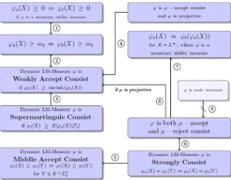
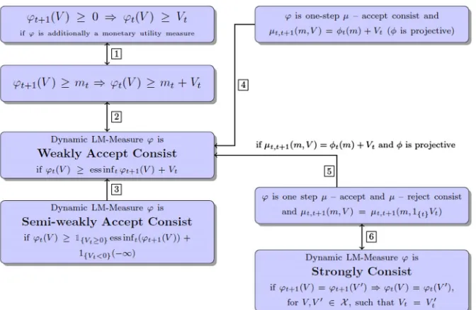
Taxonomy of results
For the convenience of the reader, in Fig. 1 below, we summarize the results sur-veyed in Section “Time consistency for random variables”. For transparency, we label (by circled numbers) each arrow (implication or equivalence) in the flowchart, and we relate the labels to the relevant results, also providing comments on converse implications whenever appropriate.
1
Proposition 2, 2) 2
Proposition 1, 4) 3
Remark 8 and Proposition 3. The converse implication is not true in general, see Example 8.