Monochromaticity of Orientation Maps in V1 Implies Minimum Variance for Hypercolumn Size

DOI 10.1186/s13408-015-0022-9

R E S E A R C H Open Access

Monochromaticity of Orientation Maps in V1 Implies

Minimum Variance for Hypercolumn Size

Alexandre Afgoustidis1

Received: 13 November 2014 / Accepted: 17 March 2015 /

© 2015 Afgoustidis; licensee Springer. This is an Open Access article distributed under the terms of the Creative Commons Attribution License (http://creativecommons.org/licenses/by/4.0), which permits unrestricted use, distribution, and reproduction in any medium, provided the original work is properly credited.

Abstract In the primary visual cortex of many mammals, the processing of sensory

information involves recognizing stimuli orientations. The repartition of preferred orientations of neurons in some areas is remarkable: a repetitive, non-periodic, lay-out. This repetitive pattern is understood to be fundamental for basic non-local as-pects of vision, like the perception of contours, but important questions remain about its development and function. We focus here on Gaussian Random Fields, which pro-vide a good description of the initial stage of orientation map development and, in spite of shortcomings we will recall, a computable framework for discussing general principles underlying the geometry of mature maps. We discuss the relationship be-tween the notion of column spacing and the structure of correlation spectra; we prove formulas for the mean value and variance of column spacing, and we use numeri-cal analysis of exact analytic formulae to study the variance. Referring to studies by Wolf, Geisel, Kaschube, Schnabel, and coworkers, we also show that spectral thinness is not an essential ingredient to obtain a pinwheel density ofπ, whereas it appears as a signature of Euclidean symmetry. The minimum variance property associated to thin spectra could be useful for information processing, provide optimal modularity for V1 hypercolumns, and be a first step toward a mathematical definition of hyper-columns. A measurement of this property in real maps is in principle possible, and comparison with the results in our paper could help establish the role of our minimum variance hypothesis in the development process.

Keywords Visual cortex·Orientation hypercolumns·Column spacing·Pinwheel density·Gaussian random fields·Kac–Rice formula

B

[email protected]

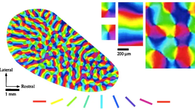
Fig. 1 Layout of orientation preferences in the visual cortex of a tree shrew (modified from Bosking et al. [10]). Here orientation preference is color-coded (for instance neurons in blue regions are more sensitive to vertical stimuli). Maps of sensitivity to different stimulus angles were obtained by optical imaging; summing these with appropriate complex phases yields Fig.1: see Swindale [11]. In particular, at singular points (pinwheels), all orientations meet (see the upper right corner); for a fine-scale experimental study of the neighbourhood of such points, see [8]

1 Introduction

Neurons in the primary visual cortex (V1, V2) of mammals have stronger responses to stimuli that have a specific orientation [1–3]. In many species including primates and carnivores (but no rodent, even though some of them have rather elaborated vi-sion [4,5]), these orientation preferences are arranged in an ordered map along the cortical surface. Moving orthogonally to the cortical surface, one meets neurons with the same orientation preference; traveling along the cortical surface, however, reveals a striking arrangement in smooth, quasi-periodic maps, with singular points known as pinwheels where all orientations are present [6–8]; see Fig.1. All these orienta-tion maps look similar, even in distantly related species [5,9]; the main difference between any two orientation preference maps (OPM) seems to be a matter of global scaling.

included for clarification purposes: we first give an intrinsic definition of the column spacing in these fields, then discuss the intervention of spectral thinness in theoretical and experimental results related to pinwheel densities. Then (Sect.2.2) we introduce the “minimum variance” property in our title, to help discuss the quasi-periodicity in the map and to try to understand better the notion of cortical hypercolumn. In the concluding Discussion (Sect.3), we also try to clarify the relevance of this property for the development of real maps and formulate a simple test for our hypothesis that it is indeed relevant.

Many models for the development of orientation maps have been put forward [5,

17–19]; they address such important issues as the role of self-organization, or of in-teractions between orientation and other parameters of the receptive profiles [14,

19–22]. In this short note, we focus on a mathematical computable framework in which geometrical properties can be discussed with full proofs, and whose quanti-tative properties can now be compared with those of experimental maps. While we thus put the focus on the geometry of theoretical maps rather than on the most real-istic developmental scenarios, we try to relate this geometry to organizing principles, viz. information maximization and perceptual invariance, which are relevant for dis-cussing real maps. In a mathematical setting, these principles can be enforced through explicit randomness and invariance structures.

Wolf, Geisel, Kaschube and coworkers [9,23–25] have described a wide class of probabilistic models for the development of orientation preference maps. In all these models (and in our discussion) the cortical surface is identified with the planeR2, and the orientation preference of neurons at a pointx is given by (half) the argument of a complex number z(x); one adds the important requirement that the mapx→z(x)

be continuous (this is realistic enough if the modulus|z(x)|stands for something like the orientation selectivity of the neurons atx; see [7,11,26]). Pinwheel centers thus correspond to zeroes of z.

A starting point for describing orientation maps in these models, one which we will retain in this note, is the following general principle: we should treat z as a random field, so at each pointx, the complex number z(x)as a random variable.

Even without considering development, it is reasonable to introduce randomness, to take into account inter-individual variability. But of the statistical properties of zero-set of general random fields, our understanding is that present-day mathematics can say very little [27]; only for very specific subclasses of random fields are precise mathematical theorems available. The most important of those is the class of

Gaus-sian Random fields [27–29]—a random field z is Gaussian when all joint laws for

(z(x1), . . . ,z(xn))∈Cnare Gaussian random variables.

stationary states of the dynamics which represent mature maps cannot be expected to be Gaussian states. We shall comment on this briefly in Sect.2.1.3and come back to it in the Discussion (Sect.3).

In spite of this, we shall stick to the geometry of maps sampled from Gaussian Random Fields (GRFs) in our short paper. We have several reasons for doing so. A first remark is that a better understanding of maps sampled from them can be helpful in understanding the general principles underlying more realistic models, or helpful in suggesting some such principles. A second remark is that with the naked eye, it is difficult to see any difference between some maps sampled from GRFs and actual visual maps (see Fig.2), and that there is a striking likeness between some theorems on GRFs and some properties measured in V1. A third is that precise mathematical results on GRFs can be used for testing how close this likeness is, and to make the relationship between GRFs and mature V1 maps clearer.

Wolf and Geisel add a requirement of Euclidean invariance on their stochastic dif-ferential equation, so that if the samples from a GRF are to be thought of as providing (early or mature) cortical maps, the field should be homogeneous (i.e. insensitive, as a random field, to a global translationx→x+a), isotropic (insensitive to a global rotation,x→cos_sin(α)(α)−_cossin_(α)(α)x) and centered (insensitive to a global shift of all orien-tation preferences, changing the value z(x)at eachxtoeiθz(x)). Here again, looking at mature maps, geometrical invariance is a natural requirement for perceptual func-tion; so we shall assume that the GRF z is centered, homogeneous, and isotropic [27,32]. Note that of course, this invariance requirement cannot be formulated in a non-probabilistic setting (a deterministic map fromR2_{toCcannot be homogeneous}

without being constant).

It actually turns out that these two mathematical constraints (Gaussian field statis-tics and symmetry properties) are strong enough to generate realistic-looking maps, with global quasi-periodicity. Quite strikingly, it has been observed [30,33] that one

needs only add a spectral thinness condition to obtain maps that seem to have the right

qualitative (a hyper columnar, quasi-periodic organization) and quantitative proper-ties (a value ofπfor pinwheel density). These mathematical features stand out among theoretical models for orientation maps as producing a nice quasi-periodicity, with roughly repetitive “hypercolumns” of about the same size that have the same struc-ture, as opposed to a strictly periodic crystal-like arrangement (see [14,21], compare [34,35]). The aim of this short note is to clarify the importance of this spectral thin-ness condition for getting a quasi-periodic “hypercolumnar” arrangement on the one hand, a pinwheel density ofπ on the other.

2 Results

2.1 Two Remarks on Gaussian Random Fields with Euclidean Symmetry

2.1.1 Preliminaries on Correlation Spectra

Let us first formulate the spectral thinness condition more precisely: in an invari-ant GRF, the correlationC(x, y)between orientations atx andy depends only on x−y. Let us turn to its Fourier transform, or rather to the Fourier components of

the mapΓ :R2→Csuch thatC(x, y)=Γ (x−y). For an invariant Gaussian field, specifyingΓ does determine the field; what is more, there is a unique measureP on R+_{such that}

Γ (τ )=

R>0

ΓR(τ ) dP (R), (1)

where, for fixedR >0, the mapΓRis1τ→

S1eiRu·τdu.

Now, correlations on real cortical maps can be measured and the spectrum ofΓ

can be inferred [30]; data obtained by optical imaging reveals that the spectral mea-sureP is concentrated on an annulus ([30, p. 100], see also [33]): this means that there is a dominant wavelengthΛ0, such that the measureP concentrates around

R0=_Λ2π

0.

Correlation spectra of real V1 maps, first discussed in [33], have been measured precisely by Schnabel in tree shrews [30] (see [30, p. 104], Fig. 5.6(d) is reproduced in Fig.2 below). The spectral measureP has a nicely peaked shape, and the very clear location of the peak is used as the dominant wavelengthΛ; see Fig.2. From Schnabel’s data we evaluate the standard deviation inP to be about 0.2Λ(caution: hereP is a real correlation spectrum, not the spectral density of a GRF).

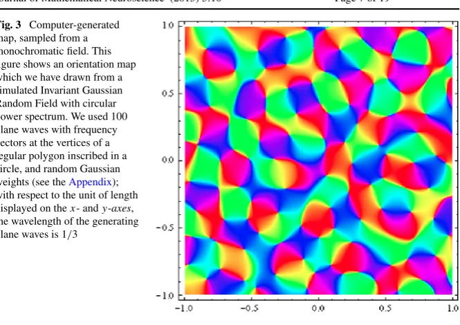
Although this is far from being an infinitely thin spectrum, it is not absurd to look at the extreme situation where we impose the spectral thinness to be zero. Figure3

shows a map sampled from a monochromatic invariant GRF, in whichΓ is one of the mapsΓR of the previous paragraph, in other words the inverse Fourier transform of the Dirac distributionδ(R−R0)on a circle: monochromatic (or almost monochro-matic) invariant GRFs yield quite realistic-looking maps, at least to the naked eye.

This thinness hypothesis certainly has to do with the existence of a precise scale in the map, that is, with the “hyper columnar” organization. In all existing theoretical studies that we know of, spectral thinness is introduced a priori into the equations precisely in order to obtain a repetitive pattern in the model orientation maps. For instance, in the very successful long-range interaction model of Wolf et al. [9,31], the linear part of the stochastic differential equation for map development features a Swift–Hohenberg operator in which a characteristic wavelength is imposed. The “typical spacing” between iso-orientation domains is then defined as that which cor-responds to the mean wavenumber in the power spectrum:

2π Λmean

:=

k dP (k). (2)

Fig. 2 Correlation spectra of orientation maps in macaque and tree shrew V1. a and b are from Niebur and Worgotter’s 1994 paper [33]: in a, the solid and dashed lines are spectra obtained by two different methods (direct measurement of correlations and Fourier analysis) from an experimental map obtained by Blasdel in macaque monkey, the power spectrum of which is displayed on b. Images c and d are from Schnabel’s 2008 thesis [30, p. 104]. Methods for obtaining c and d from measurements on Tree Shrews are explained precisely by Schnabel in [30, Sects. 5.3 and 5.4]. The green- and blue-shaded regions code for bootstrap confidence interval and 5 % significance level, respectively. The power spectrum in d has standard deviation around 0.2 in the unit displayed on the horizontal axis and determined by the location of the maximum; the mean and quadratic wavenumbers in this spectrum are in the intervals[1.05,1.10] and[1.18,1.23], respectively

2.1.2 Mean Column Spacing in Invariant Gaussian Fields

It is reasonable, both intuitively and practically, to expect thatΛmeangives the mean

local period between iso-orientation domains. For reasonable bell-shaped power spectra,Λmeanis in addition quite close to the location of the peak in the spectrum,

which very obviously corresponds to the “dominant frequency” in the power spec-trum and is quite straightforward to measure. But from a mathematical point of view, there is a paradox here.

For Gaussian fields, it is natural to try to clarify this and write down an intrinsic definition of the mean column spacing in terms of the probabilistic structure of the field. The paradox is that then the natural scale to use turns out to be different from

Λmean, and the difference is appreciable in measured spectra. We are going to show

Fig. 3 Computer-generated map, sampled from a monochromatic field. This figure shows an orientation map which we have drawn from a simulated Invariant Gaussian Random Field with circular power spectrum. We used 100 plane waves with frequency vectors at the vertices of a regular polygon inscribed in a circle, and random Gaussian weights (see theAppendix); with respect to the unit of length displayed on thex- andy-axes, the wavelength of the generating plane waves is 1/3

be the wavelengthΛsqcorresponding to the quadratic mean wavenumber:

2π Λsq :=

k2dP (k), (3)

which coincides withΛmeanif and only if the field is monochromatic.

Using Schnabel’s data to evaluate the corresponding wavelengths in real maps, we find that the quotient betweenΛsqandΛmeanis about 1.1, and they are within 15 % of each other. So using one rather than the other does have an importance.

To justify our claim thatΛsqis a good intrinsic way to define the column spacing in an invariant Gaussian field, let us consider a fixed value of orientation, say the vertical. Let us draw any lineD on the plane and look for places onD where this orientation is represented, which means that the real part of z vanishes. Now if z is an Euclidean-invariant standard Gaussian field,Re(z)|D is a translation-invariant Gaussian field on the real lineD. From the celebrated formula of Kac and Rice we can then deduce the typical spacing between its zeroes, and this yields the following theorem.

Result 1 Pick any line segment J of length on the plane and any orientation θ0∈S1. WriteNJ,θ0 for the random variable recording the number of points onJ

where the Gaussian field z provides an orientationθ0. Then

E[NJ,θ0] =_Λ

sq .

Indeed, let us writeΦ for Re(z)|D, viewed as a stationary Gaussian field on the

viewed as a homogeneous and isotropic random field onR2. The arguments lead-ing up to the statement of Result1 and the Kac–Rice formula which is recalled in theAppendixprove thatE[NJ,θ0] = ·

√

λ

π , whereλ=E[Φ(0)

2_{]. ButE[Φ(0)}2_{] =} ∂x1∂x2E[Φ(x1)Φ(x2)]|x1=x2=0, and this is∂x∂yG(x−y)|x=y=0= −G(0). To

com-plete the proof we need to calculate this.

Now, in view of the Euclidean invariance ofRe(z), we know thatG(0)is half the value ofGat zero. To evaluate this quantity, we use the spectral decomposition ofG: it reads G=_R>0GRdP (R), where GR is the covariance function of a real-valued monochromatic invariant field onR2, hence is equal to 1₂ΓR (recall thatΓR was defined in Eq. (1), and is real-valued). Now,ΓRsatisfies the Helmholtz equation

(ΓR)= −R2ΓR, and in additionΓR(0)is equal to 1, soGR(0)is equal to 1/2. We conclude thatG(0)is equal to−₄1_R>0R2dP (R)= π2

Λ2

sq. This completes the proof of Result1.

Let us now comment on this result. It means that repetitions ofθ0occur in the

mean everyΛsq. Of course this is very close toΛmeanwhen the support of the power spectrum is contained in a thin enough annulus (if the width of such an annulus is less than a fifth of its radius,ΛmeanandΛsqare within 3 % of each other). But in general, it is obvious from Jensen’s inequality thatΛmean≥Λsq, with equality if and only if the field is monochromatic. In real maps, there is an appreciable difference between

ΛmeanandΛsqas we saw.

2.1.3 Pinwheel Densities in Gaussian Fields and Real Maps

Let us turn now to pinwheel densities; we would like to comment on a beautiful the-oretical finding by Wolf and Geisel and related experimental findings by Kaschube, Schnabel and others. We feel we should be very clear here and insist that this sub-section is a comment on work by Wolf, Geisel, Kaschube, Schnabel and others; if we include the upcoming discussion it is to clarify the role of the spectral thinness condition in the proof of their result, and we seize the opportunity to comment on this work’s theoretical significance.

If a wavelengthΛis fixed, the pinwheel densitydΛin a (real or theoretical) map is the mean number of singularities in an areaΛ2. In the experimental studies of Kaschube et al. [9] and Schnabel [30], the wavelength used is obtained with two al-gorithms, one which localizes the maximum in the power spectrum, and one which averages local periods obtained by wavelet analysis. These two algorithms give ap-proximately the same result, sayΛexp, and pinwheel densities are scaled relatively to thisΛexp: a very striking experimental result is obtained by Kaschube’s group,

namely

dΛexp=mean number of pinwheels in a region of areaΛ2expπ±2 %. (4)

Theorem (Wolf and Geisel [25], Berry and Dennis [36]; see also [29,37]) Let us

writeP_A for the random variable recording the number of zeroes of the Gaussian field z in a regionA, and|A|for the Euclidean area ofA. Then

E[P_A] = π

Λ2 sq

|A|.

We think it can be of interest for readers of this journal that we include a proof of this result here. We would like to say very clearly that the discovery of this result is due to Wolf and Geisel on the one hand, and independently to Berry and Dennis in the monochromatic case. In [29], Azaïs and Wschebor gave a mathematically complete statement of a Kac–Rice-type formula, and recently Azaïs, Wschebor and León used it (following Berry and Dennis) to give a mathematically complete proof of the above theorem, though they wrote down the details only in case z is monochromatic [37]. It is for the reader’s convenience and because the focus of this short note is with non-monochromatic fields that we recall their arguments here.

Azaïs and Wschebor’s theorem (Theorem 6.2 in [29]), in the particular case of a smooth reduced Gaussian field, is the following equality:

E(P_A)= 1

2π

AE

detdz(p)|z(p)=0 dp.

Here the integral is with respect to Lebesgue measure onR2_{, and the integrand is a}

conditional expectation. To evaluate this, one should first note that z has constant vari-ance, and an immediate consequence is that for eachp, the random variable z(p)is independent from the random variable recording the value of the derivative of the real part (resp. the imaginary part) of z atp. So the random variables|detdz(p)|and z(p)

are actually independent at eachp, and we can remove the conditioning in the for-mula. Now at eachp,dz(p)is a 2×2 matrix whose columns,C1(p):=(∂xRe(z))(p)

(∂yRe(z))(p)

andC2(p):=

(∂xIm(z))(p) (∂yIm(z))(p)

, are independent Gaussian vectors (see [27, Sect. 1.4 and Chap. 5]). Because z has Euclidean symmetry,C1(p)andC2(p)have zero mean and

the same variance, sayVp, as(∂xRe(z))(p). But|detdz(p)|is the area of the paral-lelogram generated byC1(p)andC2(p), and the “base times height” formula says this area is the product ofC1(p)with the norm of the projection ofC2(p)on the

line orthogonal toC1(p). The expectation ofC1(p), a “chi-square” random

vari-able, is 2Vp and that of the norm of the projection ofC2(p)on any fixed line is

Vp; since both columns are independent, we can conclude that

E(A)= 1 π

AVpdp=

|A|

π V0

(the last equality is because z and all its derivatives are stationary fields). Now we need to evaluate V0=E{(∂xRez)(0)2}. But this quantity already appeared in the proof of Result1, it was labeled λ there. So we already proved that it is equal to

π2 Λ2

sq, and this concludes the proof of Wolf and Geisel’s theorem.

equal to π whatever the spectrum, is a rather more natural theoretical counterpart todΛexp. If we drop the focus away fromΛmeanto bringΛsqto the front, we obtain

from Result1the following reformulation of Wolf and Geisel’s theorem.

Result 2 Writefor the typical distance between iso-orientation domains, as ex-pressed by Result1, andηfor the value E[PA]

|A| of the pinwheel density. Then

η= π

2. (5)

There are two simple consequences of Wolf and Geisel’s finding which we would like to bring to our reader’s attention.

The first is that the pinwheel density ofπobserved in experiments is scaled with respect toΛexp, and not with respect toΛsq. Using Schnabel’s data, we can evaluate thedΛsqof real maps, and asΛsqis about 0.82Λexpin Schnabel’s data,dΛsqstrongly departs fromπ in real maps. Since it would be exactly π in maps sampled from GRFs, one consequence of the work in [9,25,30] is the following.

Corollary The pinwheel density of observed mature maps is actually incompatible with that of maps sampled from invariant Gaussian Fields.

This fact is quite apparent in the work by Wolf, Geisel, Kaschube, and coworkers, but since we focused on GRFs in this short note we felt it was useful to recall this as clearly as possible.

Our second remark is that in the reformulation stated as Result2here, there is no longer any spectral thinness condition. In other words, when we consider maps

sam-pled from Gaussian Random Fields, a pinwheel density ofπis a numerical signature of the fact that the field has Euclidean symmetry. Result2thus shows that when one considers invariant GRFs, average pinwheel density and monochromaticity are inde-pendent features.

Because invariant GRFs have ergodicity properties, an ensemble average such as that in Result2can be evaluated on an individual sample map; one can thus con-sider a single output of the GRF z and proceed to quantitative measurements on it to determine whether the probability distribution of z has Euclidean symmetry. Very remarkable, since no single output can have Euclidean symmetry!

To conclude this subsection, let us recall that Results1and2say nothing of map ensembles that do not have Gaussian statistics, and in particular nothing of the ge-ometry of real maps; they certainly do not mean that the definition ofΛexp used in experiments is faulty, but were simply aimed at disentangling monochromaticity from other geometrical principles in the simplified setting of GRFs. To illustrate the fact that our results are not incompatible with the definition ofΛexpused in experiments,

this time Result1-based, against GRFs representing mature maps. The measurement of the pinwheel density, Eq. (4), furthermore indicates that development seems to keep Result2true at the mature stage. We shall come back to this in the Discussion.

2.2 The Variance of Column Spacings

Results1–2show that for Gaussian Random Fields, the existence of a pinwheel den-sity of π is independent of the monochromaticity condition. We evaluated the ex-pected value of the column spacing in an invariant GRF in Result1, and we now turn to its variance. There are several reasons why it should be interesting to establish rigorously that spectral thinness provides a low variance.

A first one is the search for a mathematically well-defined counterpart to the state-ment, visually obvious, that orientation maps are “quasi-periodic”. Most mathemati-cal definitions of quasi-periodicity (like those which follow Harald Bohr [38]) are not very well suited to discussing V1 maps, and we feel that the meaning of the word is, in the case of V1 maps, well conveyed by the property we will demonstrate. While it is intuitively obvious that a “nice quasi-periodicity” should come with spectral thin-ness, as we shall see it is mathematically non-trivial.

A second reason to look at the variance is to try to understand better the concept of “cortical hypercolumn”, due to Hubel and Wiesel, which is crucial to discussions of the functional architecture of V1. Neurons in V1 are sensitive to a variety of local features of the visual scene, and a hypercolumn gathers neurons whose receptive profiles span the possible local features (note that there is no well-defined division of V1 in hypercolumns, but an infinity of possible partitionings). In studies related to the local geometry of V1 maps, once a definition for the column spacingΛhas been chosen, one is led (as in [9,24,39]) to define the area of a hypercolumn asΛ2. Here we put the focus on the orientation map only; but even then is thus legitimate to wonder whether in a domain of areaΛ2, each orientation is represented at least once. Note that a value ofπ for the pinwheel density can guarantee this if one establishes that the density also has a small variance; here, however, we are not going to evaluate this variance, which is possible in principle [37] but not easy, and we simply focus on column spacing. This is a first step in trying to check that the internal structure of domains with areaΛ2is somewhat constant, as suggested by the available results on pinwheel density.

on the sensory side corresponds to a maximum of discrimination (and Fisher informa-tion; see [40]) and on the motor side to what has been called the “minimum variance principle”, for instance in the study of ocular saccades or arm movements [41].

So we will now consider the varianceV[NJ,θ0]of the previous random variable. We will show that it reaches a minimum when the spectrum is a pure circle. Now, evaluating this variance is surprisingly difficult, even though there is an explicit for-mula, namely the following.

Theorem (Cramer and Leadbetter; see [42]) In the setting of Result1, writeG:R→

Rfor the covariance function ofRe(z)|D andM33(τ ),M44(τ )the cofactors of the (3,3)and(3,4)entries in the matrix

⎛ ⎜ ⎜ ⎝

1 G(τ ) 0 G(τ ) G(τ ) 1 −G(τ ) 0

0 −G(τ )−G(0)−G(τ ) G(τ ) 0 −G(τ )−G(0)

⎞ ⎟ ⎟ ⎠.

Then

V[NJ,θ0]

= π Λsq − π Λsq 2 + 2 π2 0 ( −τ )

M33(τ )2−M34(τ )2 (1−G(τ )2₎3/2

×

1+ M34(τ )

M33(τ )2_{−M34(τ )}2arctan

M34(τ )

M33(τ )2_{−M34(τ )}2

dτ

.(6)

Recall here that

G(τ )= 1

4π

R>0 2π

0

cosRτcos(ϑ )dϑ

P (R) dR; (7)

thisG(τ )is an oscillatory integral which involves Bessel-like functions with differ-ent parameters, and the formula forV[NJ,θ0]features quite complicated expressions using the first and second derivatives of this integral, with a global integration on top of this; so any analytical understanding of formula (6) seems out of reach! But we can check numerically that it does attest to monochromatic fields having minimum variance.

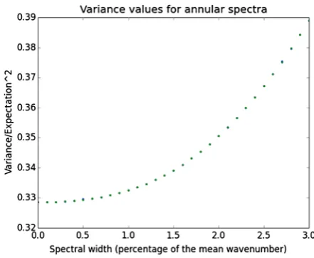
Fig. 4 Variance is a decreasing function of spectral thinness. This is a plot of the variance of the random variable recording the number of times a given orientation is present on a straight line segment of fixed length. We considered here Invariant Gaussian Random Fields with uniform power spectra, and plotted the variance as a function of spectral width. For each percentage of the mean wavenumber, we displayed two outputs to give an idea of the attained precision. A low value for variance, here expressed in the unit given by the square of the expectation, corresponds to a field whose hypercolumns have relatively constant size across the resulting orientation map; the results displayed here show that a very regular hypercolumnar organization is quite compatible with stochastic modeling, and is a direct consequence of the spectral thinness condition found in models. Moreover, the horizontal slope at zero shows that as regards the global properties of quasi-periodic maps, there is very little difference between a theoretically ideal monochromaticity and a more realistic (and more model-independent) spectral thinness

sampling strategy—and if there are multiple operations to be performed on the out-puts of these integrals—the calculations of derivatives and second derivatives of the numerically evaluatedG, and the multiple divisions, might propagate the errors quite erratically.

In order to keep the numerical errors from masking the “exact” effect of thicken-ing the spectrum, we forced the software to optimize its calculation strategy (adap-tive Monte-Carlo integration), detecting oscillations in the integrand and adapting the sampling requirements, and we extended evaluation time beyond the usual limits (by dropping the in-built restrictions on the recursion depths). When the difference be-tween successive evaluations was tamed, this yielded the variance curve displayed on Fig.4.

Note that the drawn variances correspond to fields with very slightly different spacingsΛsq; however, it is easy to check numerically that for every spectrum con-sidered here, the variance of a monochromatic field with wavelengthΛsq is inferior to the variance drawn on Fig.4.

circles of radiiRmean+0.95_Ni . We observedV[NJ,θ0]to decrease withN in that case, and the existence of a limit value. From Riemann’s definition of the integral, we see that this value is that which corresponds to a spectrum uniformly distributed in the annulus delimited byRinfandRsup. To keep the evaluation time reasonable (it is roughly quadratic inN), we kept the valueN=18 for the evaluations whose results are shown on Fig.3, and which are close to the observed limit values. We should also add here that we observed higher values for variance when using smooth spectra with several dominant wavelengths.

This is another argument for monochromaticity yielding minimum variance. Since the space of possible spectra with a fixed support is infinite-dimensional, our numer-ical experiments cannot explore it all. But we feel justified in stating the following numerical results on quasi-periodicity in orientation maps sampled from invariant Gaussian fields.

Result 3

(i) For uniform spectra, variance increases with the width of the supporting annulus. (ii) For a given spectral width, dominance of a single wavelength seems to yield

min-imum variance. Introducing more than one critical wavelength in the spectrum systematically increases nonuniformity in the typical size of hypercolumns.

Result3proves that sharp dominance of a single wavelength is the best way to obtain minimum variance. What is more, the horizontal slope at zero in Fig.3means that fields which are close to monochromatic have much the same quasi-periodicity properties as monochromatic invariant fields. This is quite welcome in view of Schna-bel’s results: of course we cannot expect actual monochromaticity in real OPMs, but clear dominance of a wavelength is much more reasonable biologically. A more theoretical benefit is the flexibility of invariant GRFs for modeling: a model-adapted precise formula for the power spectrum may be inserted without damage to the global, robust resemblance between the predicted OPMs and real maps [5].

These observations reinforce the hypothesis that our three informational principles (randomness structure, invariance, spectral thinness) are sufficient to reproduce quan-titative observable features of real maps, though as we saw, using an invariant GRF with the most realistic spectrum does not necessarily yield a more realistic result than using a monochromatic GRF, and leads to incompatibilities with the observed mature maps. This form of universality is certainly welcome: individual maps in different an-imals, from different species (with different developmental scenarii) necessarily have different spectra, but general organizing principles can be enough to explain even quantitative observed properties.

3 Discussion

whose dissemblance with real maps can be established rigorously as we recalled, we feel two new points deserve special attention: first, we showed that in the simplified setting of Gaussian Random Fields, the best mathematical quantity for explaining the local quasi-period is the quadratic mean wavenumber rather than the mean wavenum-ber, and pointed out that a pinwheel density ofπ, when scaled with respect to this intrinsic column spacing, is a signature of Euclidean symmetry and not of Euclidean symmetry plus spectral thinness; second, we established (through numerical analysis of an exact formula) that the variability of local quasi-periods is minimized when the standard deviation of the spectral wavelength tends to zero.

Our analysis shows that at least in the setting of Gaussian fields, realistically large spectra are compatible with a low variance; we suggest that a low variance for col-umn spacing might be observed in real data, and perhaps also a low variance for the number of pinwheels in an areaΛ2_exp. Spectral thinness is usually attributed to bio-logical hardware in the cortex (like pre-sight propagation wavelengths in the retina or thalamus [43,44]); this turns out to be compatible with some form of optimality in information processing.

It would also be very interesting to compare the variance of column spacings in real maps (in units of the spacing evaluated by averaging local periods) with the smallest possible value for GRFs, observed in this paper for monochromatic fields (see Fig.4); if a lower value for variance in real maps than in monochromatic Gaus-sian fields is found, it would mean that cortical circuitry refinement, featuring long-range interactions, brings mature maps closer to a geometrical homogeneity of hyper-columns. This would also throw some light on the fact that as development proceeds and the probability distribution of the field turns away from that of a GRF, driven by activity-dependent shaping, the column spacing obtained by averaging local periods seems to come closer to the wavelength associated to the mean or peak wavenumber (see [9, supplementary material, p. 5]) than it is in GRFs. It is then remarkable that development should maintain the value ofπ for pinwheel density when scaled with respect to the current value of column spacing, keeping Result2valid over time (of course the density seems to move if one does not change the definition of column spacing over time, but the best-suited quantity for measuring column spacing seems to change). Perhaps this also has a benefit for areas receiving inputs from V1, keep-ing their tunkeep-ing with the pinwheel subsystem (which seems to have an independent interest for information processing; see [45]) stable.

Competing Interests

The author declares that he has no competing interests.

Appendix

A.1 Sampling from Monochromatic Invariant Random Fields

In the main text, we defined monochromatic invariant Gaussian random fields through their correlation functions, and we studied the difference between monochromatic invariant fields and general invariant Gaussian fields. On Fig.2we displayed an OPM sampled from a monochromatic invariant Gaussian field, but we did not say how the drawn object was built from its correlation function. We provide some details in this subsection.

Recall that the covariance function of a monochromatic invariant Gaussian random field with correlation wavelengthΛis provided by the inverse Fourier transform of the Dirac distribution on a circle, that is,

C(x, y)=Ez(x)z(y)=Γ (x−y)=

S1

eiRu·(x−y)du

withR=2_Λπ. Now,Γ satisfies the Helmholtz equationΓ = −R2Γ; from this we can easily deduce that

Ez+R2z2

is identically zero. This means that any (strictly speaking, almost any) orientation map drawn from z satisfies itself the Helmholtz equation; thus OPMs drawn from

z are superpositions of plane waves with wavenumberR and various propagation directions.

Thus, we know that there is a random Gaussian measuredZon the circle which allows for describing z as a stochastic integral:

z(x)=

S1

eiRu·xdZ(u).

Now, from the Gaussian nature of z and the Euclidean invariance condition, we have a simple way to describeZ, which we used for actual computations: if(ζk)k∈N is a sequence of independent standard Gaussian complex random variables, and if

u1, . . . , un are the complex numbers coding for the vertices of a regularn-gon in-scribed in the unit circle, then

zn:x→ 1

n

n

i=1

ζieiRui·x

is a Gaussian random field. Asngrows to infinity, we get random fields which are closer and closer to a monochromatic invariant Gaussian random field, and our field

z is but the limiting field.

A.2 Kac–Rice Formula

random fields (see [29,37] and [25,27,36] in the main text). Here we give the precise theorem we used in the derivation of Result1. This formula was obtained as early as 1944, though the road to a complete proof later proved sinuous; the initial motiva-tion on Rice’s side was the study of noise in communicamotiva-tion channels, which can be thought of as random functions of time. For modeling noise it is then reasonable to introduce Gaussian random fields defined on the real line, and if the properties of the communication channel do not change over time, to assume further that they are stationary. Rice discovered that there is a very simple formula for the mean number of times this kind of field crosses a given “noise level”; this is the

Classical Kac–Rice formula Consider a stationary Gaussian Random FieldΦ de-fined on the real line, with smooth trajectories; choose a real numberu, and consider

an intervalI of length on the real line. WriteNu,I for the random variable

record-ing the number of pointsxonI whereΦ(x)=u; then

E[Nu,I] = ·

e−u2/2√λ

π ,

whereλ=E[Φ(0)2]is the second spectral moment of the field.

For the proof of this old formula, as well as a presentation of all the features of GRFs underlying our main text, see [27,42]. For the proof of the theorem we used for Result2, which is much more recent, we refer to [25] and [37].

Just after Result1, we mentioned that the comparison betweenΛmeanandΛsqis an immediate consequence of Jensen’s inequality, so let us give its statement here. We start with a continuous probability distributionPon the real line. Now whenever

ϕis a convex, real-valued function onR, Jensen’s inequality is the fact that, for each measurable functionf,

ϕ

Rf (x) dP(x)

≤

Rϕ

f (x)dP(x)

(compare the triangle inequality). In the main text, we used it whenPis the power spectrum distribution of a random field, f is the identity function of R, and ϕ is

x→x2.

References

1. Hubel DH, Wiesel TN. Receptive fields, binocular interaction and functional architecture in the cat’s visual cortex. J Physiol. 1962;160(1):106–54.

2. Hubel DH, Wiesel TN. Receptive fields of single neurones in the cat’s striate cortex. J Physiol. 1959;148(3):574–91.

3. Hubel DH, Wiesel TN. Receptive fields and functional architecture of monkey striate cortex. J Physiol. 1968;195(1):215–43.

4. Van Hooser SD, Heimel JA, Nelson SB. Functional cell classes and functional architecture in the early visual system of a highly visual rodent. Prog Brain Res. 2005;149:127–45.

6. Bonhoeffer T, Grinvald A. The layout of iso-orientation domains in area 18 of cat visual cortex: optical imaging reveals a pinwheel-like organization. J Neurosci. 1993;13:4157–80.

7. Bonhoeffer T, Grinvald A. Iso-orientation domains in cat visual cortex are arranged in pinwheel-like patterns. Nature. 1991;353(6343):429–31.

8. Ohki K, Chung S, Kara P, Hubener M, Bonhoeffer T, Reid RC. Highly ordered arrangement of single neurons in orientation pinwheels. Nature. 2006;442(7105):925–8.

9. Kaschube M, Schnabel M, Lowel S, Coppola DM, White LE, Wolf F. Universality in the evolution of orientation columns in the visual cortex. Science. 2010;330(6007):1113–6.

10. Bosking WH, Zhang Y, Schofield B, Fitzpatrick D. Orientation selectivity and the arrangement of horizontal connections in tree shrew striate cortex. J Neurosci. 1997;17(6):2112–27.

11. Swindale NV. A model for the formation of orientation columns. Proc R Soc Lond B, Biol Sci. 1982;215(1199):211–30.

12. Miller KD.π=visual cortex. Science. 2010;330:1059–60.

13. Yu H, Farley BJ, Jin DZ, Sur M. The coordinated mapping of visual space and response features in visual cortex. Neuron. 1995;47(2):267–80.

14. Reichl L, Heide D, Lowel S, Crowley JC, Kaschube M, Wolf F. Coordinated optimization of visual cortical maps (I) symmetry-based analysis. PLoS Comput Biol. 2012;8(11):e1002466.

15. Petitot J. Neurogéométrie de la vision: modeles mathematiques et physiques des architectures fonc-tionnelles. Paris: Editions Ecole Polytechnique; 2008.

16. Barbieri D, Citti G, Sanguinetti G, Sarti A. An uncertainty principle underlying the functional archi-tecture of V1. J Physiol (Paris). 2012;106(5):183–93.

17. Swindale NV. The development of topography in the visual cortex: a review of models. Netw Comput Neural Syst. 1996;7(2):161–247.

18. Chalupa LM, Werner JS, editors. The visual neurosciences. Vol. 1. Cambridge: MIT Press; 2004. 19. Nauhaus I, Nielsen KJ. Building maps from maps in primary visual cortex. Curr Opin Neurobiol.

2014;24:1–6.

20. Swindale N, Shoham D, Grinvald A, Bonhoeffer T, Hubener M. Visual cortex maps are optimized for uniform coverage. Nat Neurosci. 2000;3:822–6.

21. Reichl L, Heide D, Lowel S, Crowley JC, Kaschube M, et al. Coordinated optimization of visual cortical maps (II) numerical studies. PLoS Comput Biol. 2012;8(11):e1002756.

22. Nauhaus I, Nielsen K, Disney A, Callaway E. Orthogonal micro-organization of orientation and spa-tial frequency in primate primary visual cortex. Nat Neurosci. 2012;15:1683–90.

23. Wolf F, Geisel T. Spontaneous pinwheel annihilation during visual development. Nature. 1998;395(6697):73–8.

24. Kaschube M, Wolf F, Geisel T, Lowel S. Genetic influence on quantitative features of neocortical architecture. J Neurosci. 2002;22(16):7206–17.

25. Wolf F, Geisel T. Universality in visual cortical pattern formation. J Physiol (Paris). 2003;97(2):253– 64.

26. Nauhaus I, Busse L, Carandini M, Ringach D. Stimulus contrast modulates functional connectivity in visual cortex. Nat Neurosci. 2008;12(1):70–6.

27. Adler RJ, Taylor JE. Random fields and geometry. Berlin: Springer; 2009.

28. Abrahamsen P. A review of Gaussian random fields and correlation functions. 2nd ed. Oslo (Norway): Norsk Regnesentral; 1997 Apr. Report No.: 917. 64 p.

29. Azaïs JM, Wschebor M. Level sets and extrema of random processes and fields. New York: Wiley; 2009.

30. Schnabel M. A symmetry of the visual world in the architecture of the visual cortex [PhD thesis]. [Goettingen (Germany)]: University of Goettingen; 2008.

31. Wolf F. Symmetry, multistability, and long-range interactions in brain development. Phys Rev Lett. 2005;95:208701.

32. Yaglom AM. Second-order homogeneous random fields. In: Proceedings of the fourth Berkeley sym-posium on mathematical statistics and probability. Vol. 2, Contributions to probability theory. Berke-ley: University of California Press; 1961.

33. Niebur E, Worgotter F. Design principles of columnar organization in visual cortex. Neural Comput. 1994;6(4):602–14.

34. Koulakov A, Chklovskii D. Orientation preference patterns in mammalian visual cortex: a wire length minimization approach. Neuron. 2001;29(2):519–27.

36. Berry MV, Dennis MR. Phase singularities in isotropic random waves. Proc R Soc Lond A, Math Phys Sci. 2000;456(2001):2059.

37. Azaïs JM, León JR, Wschebor M. Rice formulae and Gaussian waves. Bernoulli. 2011;17(1):170–93. 38. Bohr HA. Almost periodic functions. New York: Chelsea; 1947.

39. Kaschube M, Schnabel M, Wolf F. Self-organization and the selection of pinwheel density in visual cortical development. New J Phys. 2008;10(1):015009.

40. Zhang K, Sejnowski TJ. Neuronal tuning: to sharpen or broaden? Neural Comput. 1999;11(1):75–84. 41. Harris CM, Wolpert DM. Signal-dependent noise determines motor planning. Nature.

1998;394(6695):780–4.

42. Cramer H, Leadbetter MR. Stationary and related stochastic processes. Sample function properties and their applications. New York: Wiley; 1967. Reprint: Dover books, 2004.

43. Ernst UA, Pawelzik KR, Sahar-Pikielny C, Tsodyks MV. Intracortical origin of visual maps. Nat Neurosci. 2001;4(4):431–6.

44. Maffei L, Galli-Resta L. Correlation in the discharges of neighboring rat retinal ganglion cells during prenatal life. Proc Natl Acad Sci USA. 1990;87(7):2861–4.