Information-Theoretic Active Perception for Multi-Robot Teams

(1)

INFORMATION-THEORETIC ACTIVE PERCEPTION FOR MULTI-ROBOT TEAMS Benjamin Charrow

A DISSERTATION in

Computer and Information Science

Presented to the Faculties of the University of Pennsylvania in

Partial Fulfillment of the Requirements for the Degree of Doctor of Philosophy

2015

Vijay Kumar, Supervisor of Dissertation

UPS Foundation Professor of Mechanical Engineering and Applied Mechanics

Nathan Michael, Co-Supervisor of Dissertation Assistant Research Professor of Robotics

Lyle Ungar, Graduate Group Chairperson Professor, Computer and Information Science

Dissertation Committee

Vijay Kumar, Professor of Mechanical Engineering and Applied Mechanics Nathan Michael, Assistant Research Professor of Robotics

Camillo J. Taylor, Professor of Computer and Information Science Daniel D. Lee, Professor of Electrical and Systems Engineering

(2)

Acknowledgements

First and foremost I want to thank my advisors, Vijay Kumar and Nathan Michael. Through-out my entire Ph.D., they gave me a great deal of freedom to pick projects that I was excited about and then provided enough concrete guidance for me to produce results. They were also invaluable in teaching me how to present ideas in papers, presentations, and conversa-tions, so that others would find our work as interesting as I do.

My entire committee also provided valuable feedback on all of my work and pushed me to make it better.

(3)

(4)

ABSTRACT

INFORMATION-THEORETIC ACTIVE PERCEPTION FOR MULTI-ROBOT TEAMS

Benjamin Charrow Vijay Kumar Nathan Michael

Multi-robot teams that intelligently gather information have the potential to transform industries as diverse as agriculture, space exploration, mining, environmental monitoring, search and rescue, and construction. Despite large amounts of research effort on active perception problems, there still remain significant challenges. In this thesis, we present a variety of information-theoretic control policies that enable teams of robots to efficiently estimate different quantities of interest. Although these policies are intractable in general, we develop a series of approximations that make them suitable for real time use.

We begin by presenting a unified estimation and control scheme based on Shannon’s mu-tual information that lets small teams of robots equipped with range-only sensors track a single static target. By creating approximate representations, we substantially reduce the complexity of this approach, letting the team track a mobile target. We then scale this approach to larger teams that need to localize a large and unknown number of targets.

(5)

List of Tables

3.1 Notation . . . 25 3.2 Measurement Model Parameters . . . 37 3.3 Computational complexity of control law . . . 38 3.4 Mean and std. dev. of RMSE of filter’s error over last 30 seconds for each

(9)

List of Figures

2.1 Entropy of a Bernoulli random variable X . . . 8

2.2 1D active perception problem . . . 14

3.1 System overview with three robots . . . 25

3.2 Normalized histograms of LOS and NLOS measurements . . . 26

3.3 Mutual information cost surface . . . 30

3.4 Starting configurations of robots . . . 35

3.5 Graphs for candidate locations . . . 37

3.6 How geometric LOS and NLOS affects nanoPAN range measurements . . . 39

3.7 Trajectories from maximizing mutual information . . . 40

3.8 Evolution of the particle filter and the robots’ movement in Experiment 1 . 41 3.9 Distance from weighted average of particles to target location using an HMM 44 3.10 Logarithm of the determinant of covariance when using an HMM . . . 44

3.11 HMM vs. Geometric . . . 44

3.12 Long Hallway and Short Hallway paths . . . 45

4.1 Representative actions for a single robot using a finite set of motion primitives with a finite horizon . . . 50

4.2 Representative actions generated by path planning . . . 50

4.3 Approximate measurement distribution. . . 54

4.4 Monte Carlo integration vs. 0th order Taylor approximation for evaluating mutual information . . . 59

4.5 Effect of approximating belief on mutual information (MI) . . . 60

4.6 Effect of approximating different beliefs on mutual information (MI) . . . . 61

4.7 Comparison of actual entropy difference to bound from Thm. 2 for mixture models that differ by one component . . . 63

4.8 Mean error of estimate for various motion primitives with 3 robots . . . 65

4.9 Indoor experimental setup . . . 66

4.10 Distance from the estimate’s mean to the target’s true location as the target drives around . . . 67

4.11 Evolution of particle filter for trial 1 of the 4 loop experiment . . . 67

5.1 Problem overview . . . 78

5.2 A single robot (orange arrow) is present in a corridor environment with two devices (black x’s) . . . 90

(10)

5.4 Time to localize all devices . . . 94

6.1 Mutual information vs. CSQMI . . . 100

6.2 Beam based measurement model . . . 101

6.3 Nearly independent beams . . . 105

6.4 Planning paths to view frontier clusters. Occupied voxels in the map are colored by their z-height. (a) Detected and clustered frontier voxels at the end of the hallway (top of the figure). (b) Poses where a robot can view one cluster are shown as red arrows. (c) The shortest path from the robot’s location (bottom of the figure) to one of the sampled poses is shown as a blue line. (d) Paths that view all clusters. To plan all paths simultaneously, first build a lookup table of where each cluster can be viewed (Alg. 3), and use it while running Dijkstra’s algorithm to plan single source shortest paths. . . . 107

6.5 Independence leads to overconfidence . . . 109

6.6 Percentage increase in CSQMI for a single beam observing the same cells over multiple time steps . . . 109

6.7 Ground robot results using CSQMI . . . 110

6.8 Time to evaluate the information of a single beam . . . 110

6.9 Quadrotor results . . . 114

7.1 Local and global planning with trajectory optimization . . . 118

7.2 Results with ground and air robots . . . 119

7.3 System architecture . . . 121

7.4 Global Planning . . . 122

7.5 Information gain performance on recorded data . . . 126

7.6 Ground robot experiments . . . 128

7.7 Planning times on recorded data . . . 129

7.8 Aerial robot stairwell simulations . . . 130

7.9 Limitations . . . 132

8.1 Limitations of planning over a finite time horizon . . . 135

8.2 System architecture for a 2 robot team . . . 136

8.3 HMDMTSP to GTSP . . . 140

8.4 Creating an HRRP instance . . . 143

8.5 Simulated Skirkanich Hall . . . 147

8.6 Cooperative mapping . . . 148

8.7 Entropy Reduction . . . 149

8.8 Time to solve HRRP . . . 149

(11)

Chapter 1

Introduction

Gathering information quickly and efficiently is a fundamental task for many real-world applications of robotics. Inspecting ship hulls for structural defects [36], building 3D models of damaged buildings [83], determining which crops need to be irrigated [2], and localizing devices in smart buildings [107] are all examples of information gathering tasks with broad commercial applicability. At their core, they are “active perception” problems which require robots that can both estimate quantities of interest and autonomously take actions to improve those estimates [4].

Teams of robots are particularly appealing for these types of problems. Unlike individual robots, they can obtain multiple sensor measurements from different places at the same point in time. When each robot is only equipped with sensors that provide limited information like RF antennas, teams are able to estimate quantities that an individual robot cannot. Even when using information rich sensors like cameras and laser range finders, the time it takes to gather information can decrease super-linearly with the size of the team [134]. Different types of robots also often have substantially different capabilities in terms of available sensors, where they can move, and how long they can be active before they run out of power. Consequently, teams comprised of heterogeneous robots are more capable than any individual robot.

(12)

chal-lenging problem that encompasses many different areas of robotics research. For example, robots must be capable of autonomously navigating to various parts of an environment. This requires robots that are capable of planning paths that do not collide with obstacles or other robots and using controllers that can generate inputs to actuators such that robots follow those paths. Navigation also requires that each robot is capable of determining where it is in space, a task known as localization. Depending on whether or not the robots are op-erating in an environment whose essential structure is known, robots may also need to solve the mapping problem, which requires them to build a detailed model of the environment they are in. In addition to all of these tasks, active perception problems require robots to estimate external quantities such as the location of a lost piece of medical equipment or the exact geometry of a building. As much as possible, a team of robots must effectively coordinate its actions.

Although each of these subproblems is challenging in its own right, the primary focus of this thesis is on principled and computationally efficient information gathering strategies for multi-robot teams. In the remainder of this chapter, we discuss some of the primary research challenges in designing such strategies. We then summarize the remainder of this thesis which describes a series of active perception problems and corresponding strategies to solve them.

1.1 Research Problems

(13)

that we want any strategy to exhibit:

1. General. Given the wide variety of active perception problems, it is desirable to de-velop algorithms that generalize across different sensing modalities and enable robots with different mobility constraints to reduce an estimate’s uncertainty as much as possible.

2. Clarifying. The faster robots can obtain low uncertainty estimates the better. This means that an approach should take actions that are likely to reduce an estimate’s uncertainty.

3. Online. Robots continuously gather measurements as they take actions, enabling them to gradually form more certain estimates. An active perception approach should be able to take advantage of this increased information and adapt its actions to exploit everything that it knows.

4. Collaborative. An estimate’s uncertainty can often be reduced faster by effectively coordinating multiple robots. Strategies that can achieve this are preferable to those that can’t.

Developing a control policy that achieves all of these goals is difficult. Strategies that use approximations and simplified models may be quick to compute, but the selected actions may not substantially reduce the uncertainty of the estimate. Conversely, robots may be able to use detailed probabilistic models to predict how their actions are likely to improve the estimate. Unfortunately, given the inherent uncertainty in these predictions, computing these policies can take a long time. This issue is particularly important in time-critical scenarios such as search and rescue.

Although there are many different types of active perception problems, there are two broad classes that can be addressed: estimating low-dimensional state with low-information sensors and estimating high-dimensional state with high-information sensors.

(14)

angle between a robot and the target). In addition to being a challenging active perception problem, range-only target localization can also be used to solve real world problems. For example, in the near future, automated buildings will use a large number of devices for a variety of services including power and water monitoring, building security, and indoor localization for smart phones [107]. Effectively using and maintaining this many devices will require knowing where each of them is located. A cost-effective way of getting this informa-tion would be to equip each device with RF or audio based range-only sensors [74, 99]. This approach could even work when sensors are embedded in a building’s walls [43]. Because range-only sensors only provide limited information about a device’s location and having humans localize all devices would be a time consuming and error prone task, it is natural to try and automate the process using a team of robots.

On the opposite extreme of active perception are problems like active mapping which require robots to build a complete and low uncertainty model of the environment that they are operating in. These maps typically consist of probabilistic estimates of the presence and location of obstacles and require the use of sensors like laser-range finders or 3D cameras like the Microsoft Kinect. Active mapping is then a problem that involves estimating high-dimensional state with high-information sensors. Being able to autonomously construct these maps has a large number of potential applications like inspecting ship hulls for defects or mines [36], exploring the surface of other planets [30], and assisting in disaster relief by giving safety workers a clear idea of how buildings are damaged [83].

(15)

collaboration strategies. In range-only localization teams can reduce uncertainty faster by gathering multiple measurements to the same target, but in active mapping they can often reduce uncertainty faster by observing different parts of the map.

1.2 Thesis Overview

The primary goal of this work is to develop computationally tractable information-theoretic control laws that enable multi-robot teams to effectively coordinate their actions to gather measurements that reduce the uncertainty of estimates. This thesis makes a variety of contributions that make substantial progress towards solving the research problems outlined in the previous section:

1. Ch. 3 introduces a basic form of the range-only localization problem, in which a small team of robots must localize a single static target in a known environment. We develop an accurate estimation scheme for a commercially available RF range-only sensor as well as a mutual information based control law.

2. Ch. 4 develops techniques for approximating mutual information, enabling it to be calculated substantially faster. This enables the approach from Ch. 3 to track a mobile target, by enabling the team to consider the impact of multiple measurements over time while planning, going beyond a greedy one-step maximization. Importantly, we prove that the approximations introduce bounded error. This proof also bounds the difference in mutual information between different control inputs, which makes it easier to generate appropriate actions.

3. Ch. 5 extends the range-only problem to the case where a team of robots must localize an unknown number of targets throughout an environment. It also addresses the exponential complexity inherent in multi-robot planning problems, enabling larger teams of robots to effectively work together. The computational complexity of the resulting control strategy is polynomial in all relevant variables.

(16)

to many other approaches, we explicitly model the dependence of separate measure-ments over multiple time steps to develop online algorithms that search over multiple, multi-step actions. This chapter also examines how information-theoretic control laws generalize across different platforms by conducting experiments where individual air and ground robots map different environments.

5. Ch. 7 shows how a hierarchical planning framework combined with trajectory opti-mization can substantially improve the performance of active mapping strategies, by enabling robots to quickly compute feasible and locally optimal information-theoretic trajectories.

(17)

Chapter 2

Background and Related Work

This chapter introduces the basic concepts of information theory and how it can be used to develop an active perception control law. It also surveys recent research in active perception that is relevant to this thesis.

2.1 Information Theory

Information theory was developed in the 1940’s by Shannon [115] and others. Shannon’s work was motivated by designing ways to encode, transmit, and decode messages without them being corrupted by noise.

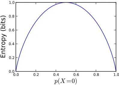
One fundamental contribution of the theory is Shannon’s entropy, a general measure of the uncertainty of a random variable. For a discrete random variable X, that can take values in the set X ={x1, . . . , xN}, Shannon’s entropy is defined as:

H[X] =Ep(X)[−log2p(X =x)] =−

X

x∈X

p(X =x) log₂p(X=x) (2.1)

In general, H[X] is non-negative and 0 if and only if X is not random (i.e., takes a value with probability 1). The units of Shannon’s entropy are bits when the base of the logarithm is 2 and nats when the natural logarithm is used.

(18)

0.0 0.2 0.4 0.6 0.8 1.0

p

(

X

=0)

0.0 0.2 0.4 0.6 0.8 1.0

Entropy (bits)

Figure 2.1: Entropy of a Bernoulli random variableX.

value is sensible, as a single bit can encode two different values, and both outcomes are equally likely. For comparison, supposeB is a biased coin wherep(B =Heads) = 0.99 and

p(B =T ails) = 0.01. B’s entropy is H[B] = 0.08 bits. This is also a sensible value as the outcome of B is quite certain; we would be surprised if we got a tails. Fig. 2.1 shows that the entropy of a generic Bernoulli random variable. As one would hope for a measure of uncertainty, entropy is highest when the outcome is most uncertain, and gradually decreases to 0 as the outcome becomes more certain.

Shannon’s entropy can be extended by analogy to continuous distributions. If X is a continuous random variable, then itsdifferential entropy is:

H[X] =Ep(X)[−logp(X=x)] =−

Z

p(X=x) logp(X =x)dx (2.2)

Unlike discrete entropy, differential entropy can be negative. While it has a similar form to discrete entropy, it is not the limit of discrete entropy, and in fact differs by an infinite offset [27]. Despite this, differential entropy is similar conceptually, and we will use the two concepts interchangeably. As many quantities in robotics are continuous, most of the work in later chapters uses differential entropy.

(19)

we have two random variables X and Z, and we want to know the entropy of X given

Z. This would be straightforward if Z were known; it would simply be the entropy of the distributionp(X |Z =z). However,Z is also a random variable, so we take an expectation over it:

H[X|Z] =Ep(Z)[H[X|Z =z]] (2.3)

=X

z∈Z

p(Z =z) −X

x∈X

p(X=x|Z =z) log₂p(X=x|Z=z)

!

(2.4)

Similar to differential entropy, conditional differential entropy can be defined for continuous random variables by replacing the appropriate sums with integrals.

Together, entropy and conditional entropy can be used to measure the likely decrease in uncertainty of a random variable. This quantity is known as mutual information:

IMI[X;Z] = H[X]−H[X|Z] (2.5)

= H[Z]−H[Z |X] (2.6)

Note that for both discrete and continuous distributions, mutual information is always non-negative and 0 if and only if the two random variables are independent. The non-negativity has an interesting interpretation that “information never hurts” [27]; learning the outcome of a random variable cannot increase uncertainty.

One important property of mutual information is that it can be expressed in two different ways. In other words, each random variable contains the same amount of information about the other. This is helpful, because whenZ is the measurement andX is the state,p(Z |X) is the measurement model, which can often be modeled in robotics. This makes (2.6) easier to calculate than (2.5), as (2.5) requires calculatingp(X |Z) which is either the posterior distribution or an approximate inverse measurement model [134].

(20)

satisfy. For example, one requirement is that the uncertainty of independent events must be the sum of the uncertainty of the individual events. Shannon described five axioms and proved that (2.1) is theonly definition of uncertainty that satisfies all of them.

However, there are alternative axiomizations of uncertainty, notably by Renyi [104]. These measures only satisfy some of Shannon’s axioms, but still provide useful characteri-zations of uncertainty. Renyi’s α-entropy for continuous random variables is defined as:

Hα[X] =

1 1−αlog

Z

pα(X=x)dx (2.7)

Anyα >1 including α→ ∞ results in a valid entropy. In the limit asα goes to 1, Renyi’s entropy converges to Shannon’s entropy [100].

Our primary motivation for studying alternative forms of uncertainty is that Shannon’s entropy and mutual information are hard to compute, except in certain special cases like Gaussian models. The source of this difficulty is the expectation over the logarithm in (2.1), which frequently prevents the integral from being evaluated analytically. For this reason, Renyi’s quadratic entropy (RQE), also known as the collision entropy, is particularly interesting:

H2[X] =−log

Z

p2(X =x)dx (2.8)

As noted by Principe [100], this form is computationally useful because 1) the logarithm appears outside the integral and 2) when p(X) is a Gaussian or a Gaussian mixture model, the integral can be calculated analytically, because all of the integrals are the products of Gaussians.

(21)

defined as:

DKL[f ||g] =Ef[logf /g] =

Z

f(x) logf(x)

g(x) dx (2.9)

KL divergence is non-negative and 0 if and only iff andg are equal almost everywhere. In general, it is not symmetric (i.e., DKL[f ||g]6= DKL[g||f]) and does not obey the triangle inequality, making it a pseudo-metric [27]. Interestingly, the mutual information of two variablesX and Z, can be expressed as the KL divergence between their joint distribution,

p(X, Z), and the product of their marginal distributions,p(X)p(Z):

IMI[X;Z] = DKL[p(X, Z)||p(X)p(Z)] (2.10)

Because p(X, Z) =p(X)p(Z) if and only ifX and Z are independent, mutual information can be viewed as a measure of how dependentX and Z are. If they are independent, then there is no difference between the product of the marginals and the joint distribution, so their mutual information is 0. But if X and Z are very dependent – the outcome of one random variable changes likely outcomes of the other – then their mutual information will be high.

Viewing information as a measure of dependence between random variables makes it easier to define alternative measures of information. Specifically, we can define a new notion of information by replacing KL divergence in (2.10) with a different probability measure. Gibbs and Su [44] provide a good survey of different metrics and how they are related. Principe [100] also discusses several different options. Of particular interest is the Cauchy-Schwarz divergence (CS divergence), which for two densities f and g is defined as:

DCS[f ||g] =−log

Z

f(x)g(x)dx

2

Z

f2(x)dx

Z

g2(x)dx

(2.11)

(22)

that it is non-negative and 0 if and only if the densities are equal almost everywhere [100]. It can be used to define the Cauchy-Schwarz quadratic mutual information (CSQMI) between random variables:

ICS[X;Z] = DCS[p(X, Z)||p(X)p(Z)] (2.12)

There is a connection between CS divergence and Renyi’s quadratic entropy that is quite similar to the relationship between KL divergence and Shannon’s entropy. This similarity then links mutual information and CSQMI. KL divergence can be written in terms of Shannon’s cross entropy and Shannon’s entropy:

DKL[f ||g] =−Ef[logg]−H[f] (2.13)

The cross entropy, Ef[−logg], measures the efficiency of encoding a message using a

dis-tribution given by g rather than the true distribution f. Similarly, Rao [102] showed that CS divergence can be expressed as:

DCS[f ||g] = (−logEf[g]−H2[f]) + (−logEg[f]−H2[g]) (2.14) H2[·] is Renyi’s quadratic entropy, and −logEf[g] can be viewed as Renyi’s quadratic cross

entropy. The grouped terms are thus completely analogous to KL divergence, suggesting that CSQMI and mutual information express similar concepts.

(23)

what is intended.

We defined all of the concepts in this section in terms of random variables, but the definitions for random vectors are nearly identical. The only change is that the domain and dimensionality of the probability mass and density functions increases. This is useful as it gives us a consistent notation for handling all cases. When it makes the presentation clearer, we will use boldface to denote vector quantities.

2.2 Information Based Control for Robotics

Given its basis as a theory of communication, information theory may not seem connected to active perception. However, the fundamental goal of active perception is to reduce uncertainty of an estimate, and information theory provides many ways to quantify this intuitive notion. In this section, we use a simple range-only localization problem to explain how information theory can be applied to active perception. The work presented in later chapters will formalize and expand this approach, but the fundamental ideas will remain the same.

A generic estimation problem is to estimate some state, x, given a sequence of measure-ments taken from time 1 to time t: [z1, . . . , zt] = z1:t. The posterior distribution over the

state is p(x | z1:t). At time t, the robot must take an action to obtain a better estimate

of x. If the state of the robot is c, then the measurements that it gets should depend on the true state as well as the robot’s position; the measurement model – distribution over measurements – can be specified asp(z|x, c). After the robot takes an action, it will get a new measurement, update its estimate, repeat the process. One reasonable control policy is to select an action that will likely result in the smallest entropy (i.e., uncertainty) of the posterior estimate at timet+ 1. Formally, given a set of possible actionsA={a1, . . . , aN},

this control policy would be:

a∗ = arg min

a∈A

H[x|zt+1, z1:t, a] (2.15)

(24)

d1 d2

(a)

d1 d2

(b)

d1, d2 z

p

(

z

)

(c)

d1 d2

z

p

(

z

)

(d)

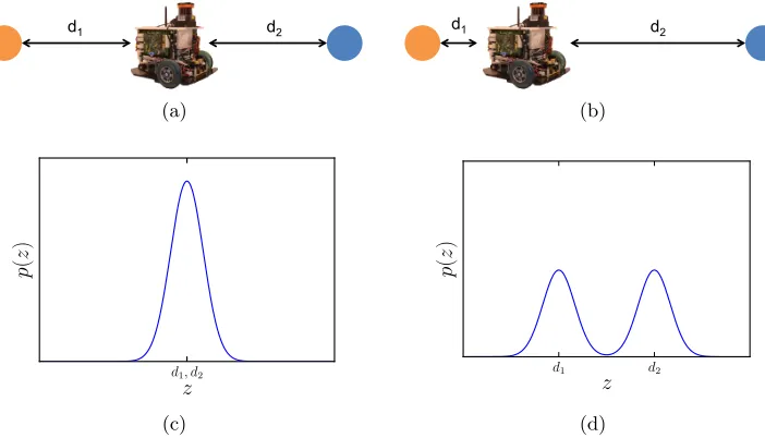
Figure 2.2: 1D active perception problem. (a) Orange and blue dots show two possible locations for a target. When the robot is equidistant from both, d1 = d2, the robot can predict that future measurements, (c), will not help distinguish between the two hypotheses. (b) and (d) show that the robot can predict that moving closer to one hypotheses is a better choice, because the received measurement depends on the target’s true location.

variables), whereas x andzt+1 are unknown as they’re in the future.

Minimizing the conditional entropy of the future estimate, (2.15), is equivalent to max-imizing mutual information. Using (2.5):

arg min

a∈A

H[x|zt+1, z1:t, a] = arg min a∈A

H[x|z1:t]−IMI[x;zt+1 |z1:t, a] (2.16)

= arg max

a∈A

IMI[x;zt+1 |z1:t, a] (2.17)

This equivalence serves as the primary motivation for maximizing mutual information and other quantities that measure the dependence between random variables.

(25)

the distribution over measurements that it is likely to receive using the marginalization rule of probability: p(z | a) = R

p(x)p(z | x, a)dx. Fig. 2.2c and Fig. 2.2d show the distribution over measurements that the robot can predict at the current time t. Due to the symmetry of the target’s position in Fig. 2.2c, the uncertainty of the measurements, H[z], is due to the uncertainty inherent in the sensor itself. As this uncertainty is given by H[z|x], H[z] = H[z|x], meaning the mutual information is close to 0. In contrast, the uncertainty of measurements in Fig. 2.2d is substantially higher, due to the fact that it’s unclear whether the robot is close to or far from the target. In this case H[z]>> H[z|x], so mutual information will be high. Consequently, an information based strategy will pick the action that brings it closer to the target, which is the better choice.

The simple 1D example illustrates the benefits of using an information based control policy. A primary advantage is that because this approach uses the same probability models as the estimation process, it naturally accounts for sensor limitations like noise or limited field of view. Additionally, maximizing information naturally extends to multiple time steps, robots, and sensing modalities, as each of these have well defined effects on the posterior distribution.

The 1D example also illustrates some of the drawbacks of information. While the ex-pressions are quite general, they are difficult to compute, as they require integrating over the joint state and measurement spaces. Except in more restricted settings like linear-Gaussian models, the requisite integrals are difficult to evaluate. Developing appropriate approximations and measures to avoid these issues is a central focus of this thesis.

2.3 Limited Information Active Perception

There is extensive work on estimation and active perception for limited sensing domains. Two widely studied problems are range-only localization and bearing-only localization.

(26)

handling disturbances to Ultra-Wideband (UWB) radios that are caused by line-of-sight conditions and different construction materials. Researchers have also examined situations where the target is moving. For example, Hollinger et al. [54] studied how to estimate a mobile target with fixed and uncontrollable range radios. While the preceding approaches used a Bayesian filter to obtain estimates, researchers have also formulated range-only es-timation as a non-linear optimization problem [88] or a spectral learning problem [9]. For active perception, using a recursive Bayesian filter for estimation has the advantage of pro-viding an up to date belief at each point in time. All of these works used a human operator to manually drive a robot to gather measurements.

Given that estimation often produces probabilistic estimates, many researchers have formulated the active perception problem as an optimization of some information-theoretic quantity. Grocholsky [49] and Stump et al. [132] designed controllers which maximized the rate of change of the Fisher information matrix (FIM) to localize a stationary target. As the FIM lower bounds the covariance (i.e., uncertainty) of any unbiased estimator [27], minimizing its inverse enables better estimates. However, this work assumed that the belief is Gaussian, which is not the case for typical range measurements. More recently, Levine et al. [77] looked at how to combine the FIM with rapidly-exploring random trees to plan informative paths for robots with non-trivial dynamics. Mart´ınez and Bullo [81] also examined using the determinant of the FIM for target tracking.

(27)

approximations enable us to calculate control inputs for multiple robots in real-time. In probabilistic estimation problems, it is often difficult to obtain theoretical guarantees about the performance of an active control policy. One exception is Vander Hook et al. [137], who developed an approach for a single target bearing-only sensor problem. They proved that the time it takes their approach to decrease the covariance of the estimate by any given factor is constant factor competitive with any active control policy. While this result is limited to bearing-only sensors and open environments where a robot can move freely, it is still an interesting guarantee, particularly as the bound is with respect to time. The focus of this thesis is different, as we develop algorithms for teams of robots with a variety of sensors that take intelligent actions even when their movement is constrained.

Any active control policy faces the question of how to parameterize the actions the robots can take. One popular approach is to use motion primitives, which has the advantage that the objective only needs to be computed over a discrete set and can be used to incorporate other properties such as obstacle avoidance. However, it is often possible to locally optimize an initial action for the robots by considering the gradient of an objective. Spletzer and Taylor describe a sampling based method for evaluating the gradient of several different types of objectives [126, 125] while Schwager et al. [112] give an explicit characterization of the gradient of mutual information with respect to the configuration of the team.

(28)

formaliza-tion allows them to provide guarantees on the rate of convergence for their active search procedure. Geometric and probabilistic strategies are not mutually exclusive. For exam-ple, Schwager et al. [113] examined different ways of combining geometric and probabilistic objectives.

A number of researchers have studied issues relating to communication. Kassir et al. [68] developed a distributed information-based control law that explicitly modeled the cost of sending data between agents. In a range-only tracking problem, they showed how their algorithm reduced the amount of inter-agent communication in a Decentralized Decision Making algorithm without significantly affecting the system’s overall performance. In re-lated work, Gil et al. [45] developed a controller to position a team of aerial robots to create a locally optimal communication infrastructure for a team of ground robots. Julian et al. [64] developed distributed algorithms for calculating mutual information to estimate the state of static environments using multi-robot teams.

(29)

2.4 Information Rich Active Perception

Information rich problems are those where a robot must estimate high dimensional state. A prototypical example of this problem is active mapping, for which there is a considerable body of prior work [133, 128]. One key question for any active mapping approach is how to represent a static map of the environment. Such representations include, but not limited to, topological maps, landmark-based representations, elevation grids, point clouds, meshes, and occupancy grids [134].

Given a map representation, strategies for mapping and exploration can be primarily grouped into two categories: (i) Frontier-based, and (ii) Information-gain based strategies. Frontier-based strategies [142] are primarily geometric in nature and travel to the dis-crete boundary between the free and unknown regions in the map. Extensions of this strat-egy have been successfully used for building maps of unknown environments in 2D [47, 12]. Holz et al. [56] provide a comprehensive evaluation of frontier-based strategies in 2D envi-ronments. Direct extensions to voxel grid representations of 3D environments using frontier voids have also been proposed [42, 35]. Shade and Newman proposed a combination of a frontier-based and a local vector-field based strategy to generate shorter exploration trajec-tories [114]. Although they do not compute frontiers directly, Shen et al. [117] used a similar strategy with a particle-based representation of free space for computational tractability. While frontiers are somewhat difficult to use in 3D environments [117], they do provide a useful way to generate potential actions for information-theoretic objectives [129].

(30)

use a greedy controller with a one-time step look ahead. Soatto [123] suggests planning over multiple time steps to deal with the issue of a greedy explorer getting stuck in local minima. To address this issue, researchers have proposed considering a discrete set of actions and executing the one that maximizes information gain [10, 40]. Rocha et al. [105] use the gradient of map entropy to select promising frontiers for exploration. These strategies do not locally optimize the robot trajectory with an intent to gain more information as the robot is traveling to the next selected frontier, which might result in inefficient mapping behavior.

Prior work has used trajectory optimization over a finite horizon to optimize information-theoretic criteria [90, 24, 110, 80]. However, these approaches have been primarily limited to continuous representations of the belief and measurements.

One drawback to many frontier-based and information-based strategies is that they only plan over a finite horizon. Particularly when a robot must travel to every destination in an environment, this can result in the robot repeatedly traversing the same parts of an environment in order to observe everything. When an uncertain but complete prior estimate is available, coverage strategies, which are geometric in nature, avoid this issue by planning paths that will observe every portion of the environment. Englot and Hover [36] developed such a strategy to build a detailed model of a ship’s hull. Kollar and Roy [71] adopted a similar approach and framed exploration as a constrained optimization problem, but learned to predict how trajectories would reduce the robot and map’s uncertainty using reinforcement learning.

(31)

reduce the uncertainty of the robot’s state and the map [10, 129, 136, 69, 60]. Stachniss et al. [129] also considered the active SLAM problem. Using a Rao-Blackwellized particle filter to estimate the joint distribution over maps and the robot’s trajectory, they proposed selecting actions that maximize the expected reduction in the filter’s entropy, accounting for uncertainty in the robot’s pose as well as the uncertainty of the map. However, this approach is expensive, as it requires calculating entropy by repeatedly copying the filter and updating it with a randomly sampled measurement.

For planning approaches that seek to maximize mutual information, one important ques-tion is how close to optimal they are. Although these problems are typically NP-hard, build-ing on work in combinatorial optimization by Nemhauser et al. [87], Krause and Guestrin [72] derived approximation guarantees for greedy maximizations of mutual information and other submodular set functions. These results were applied to mobile robot environmental monitoring problems by Singh et al. [119] and Binney et al. [7]. These guarantees only hold in offline settings where teams do not update their actions based on measurements they receive. Golovin and Krause [46] generalized these ideas to online settings, deriving performance guarantees for adaptive submodular functions. Unfortunately, these guaran-tees require all actions to be available to all robots at all times, making them not directly applicable to the problems discussed in this thesis. Hollinger and Sukhatme [53] develop a sampling based strategy for maximizing a variety of information metrics with asymptotic optimality guarantees. However, they assume that information is additive across multiple measurements (i.e., measurements are independent). This assumption limits cooperation in multi-robot settings (Ch. 3) and can lead to overconfidence when considering multiple measurements of the same quantity (Ch. 6). Unlike the guarantee provided by Vander Hook et al. [137], these guarantees are all with respect to an objective like mutual information and not a performance metric like time to reduce uncertainty by a given amount.

(32)

visual servoing [28], and active object modeling [140]. They have also been used for ap-plications outside of active perception. For example, Kretzschmar and Stachniss [73] use mutual information as a criterion for storing a minimal number of laser scans toward map reconstruction.

(33)

Chapter 3

Estimation and Control for

Localizing a Single Static Target

Having robotic teams that are capable of quickly localizing a target in a variety of environ-ments is beneficial in several different scenarios. Such a team can be used in search and rescue situations where a person or object must be located quickly. Cooperative localiza-tion can also facilitate localizalocaliza-tion of robots within a team towards tasks like cooperative mapping or surveillance. Given these multiple applications, it is reasonable to equip the robots with additional sensors to support localization. In this chapter, we focus on the case where each robot is equipped with a range-only radio frequency (RF) sensor. These sensors provide limited information about the state of the target, necessitating the development of an active control strategy to localize it.

This chapter makes two primary contributions. The first is an experimental model for radio-based time-of-flight range sensors. The second is a general framework for active control which maximizes the mutual information between the robot’s measurements and their current belief of the target position. Both of these pieces serve as building blocks for Ch. 4 and Ch. 5, which extend the approach to consider the effect of multiple measurements, larger teams, and to scenarios with mobile or multiple targets.

(34)

communication throughout the team. This limitation is typically not significant in the sce-narios we consider as the team’s only sensor is RF-based. If the team was in an environment where they could not communicate, they could not gather measurements either.

In the rest of this chapter we detail the estimation and control algorithms that enable a team of robots to successfully localize a single stationary target in non-convex environments. Our primary focus is on a series of experiments that we designed to test the approach across different indoor environments and a variety of initial conditions. Overall, we are able to repeatedly localize a target with an error between 0.7−1.6 m using only two robots equipped with commercially available RF range sensors. A highlight of this work is that despite the limited information that the team has when they are at any fixed position, they are able to effectively coordinate and use their mobility so that the estimate of the target rapidly converges.

This chapter originally appeared in [14, 17].

3.1 Technical Approach

In our approach, the robotic team maintains a distribution over possible locations of the target’s location using a particle filter. The team constantly seeks to maximize the mu-tual information between the current estimate of the target’s state and expected future measurements. Both the filter and the control directions are computed in a centralized manner as illustrated in Fig. 3.1. This approach could be made tolerant to some types of communication limitations similar to the system presented by Dames and Kumar [29].

3.1.1 Measurement Model

(35)

Table 3.1: Notation.

Symbol Description

x Mobile target’s 2D position

z Range measurements

t Current time

σ2

m Measurement noise

σ2

p Process noise

c Destinations for the

team

T Length of future time

interval

R Size of team

M Num. of particles for

target prediction

Target

Es*ma*on Predic*on Target

Team Trajectory Genera*on Range sensing

Naviga*on Robot 1

Robot 2

Robot 3

Control Law

Range sensing

Naviga*on

Range sensing

Naviga*on

Figure 3.1: System overview with three robots. In this ex-ample, Robot 3 aggregates range measurements and estimates the location of the target. This estimate is used to predict the target’s future locations over several time steps. The control law selects the trajectory that maximizes the mutual informa-tion between the target’s predicted locainforma-tion and measurements the team expects to make. This trajectory is sent to the other robots which follow it.

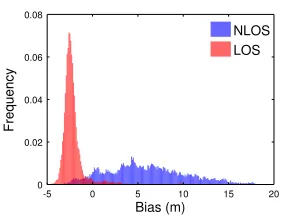
biases, which are primarily a function of whether or not the sensors are in line of sight (LOS) or non line of sight (NLOS). Our data also show that the magnitude of the bias and variance increase with the true distance between the sensors.

There is significant empirical and theoretical support for treating LOS and NLOS mea-surements differently [103, 99]. Fig. 3.2 shows a histogram of biases which demonstrates this. RTT methods work best when radios are not obstructed by obstacles and have clear LOS conditions. However, when radios do not have LOS they are more likely to be affected by scattering, fading, and self-interference, causing non-trivial positive biases. We model the error of the measurement conditioned on the true state as:

p(z|x) =

      

N(z;α0+rα, rσL2) LOS

N(z;β0+rβ, rσ_N2 ) NLOS

(3.1)

(36)

Bias (m)

Frequency

-5 0 5 10 15 20

0 0.02 0.04 0.06 0.08

NLOS LOS

Figure 3.2: Normalized histograms of LOS and NLOS measurements. Both histograms have 20,000 measurements. LOS measurements typically underestimate distance (negative bias), while NLOS overestimate it (positive bias).

true state (i.e.,p(z1, z2 |x) =p(z1 |x)p(z2 |x)).

Models for TDoA sensors typically use a biased Gaussian with constant or time-varying variance [111, 62], whereas (3.1) is more similar to those used in power based range models. We have chosen this approach because, as Patwari et al. noted, the Gaussian model does not perform as well at large distances as the tails of the distribution become heavy [99]. Letting the variance increase with distance ensures that the model handles large deviations from the truth without using a Gaussian mixture model, which would increase the computational complexity of the control as we discuss later.

Because the error statistics of LOS and NLOS measurements are so different, it is important to correctly classify measurements. Using the wrong model to incorporate mea-surements can result in the filter converging to an incorrect location of the target.

One approach – assuming the robots have a map of the environment – is to usegeometric LOS and check if a raycast between a hypothesized target location and the measuring robot intersects any walls. This works well with particle filters as measurements can be classified on a per particle basis.

The primary drawback to the geometric approach is that geometric LOS can be different from RF LOS. As we show experimentally, measurements can have a negative bias and relatively low variance – indicating RF LOS – even when the target and robot do not have geometric LOS.

(37)

measurements based on their observed mean and variance. By using the statistics of the measurements, the HMM typically differentiates RF LOS and RF NLOS more accurately than the geometric method because it does not rely on the assumption that geometric LOS predicts RF interference. Concretely, we model noise as a two state HMM with non-distance dependent Gaussian emissions. To classify a group of measurements, we subtract their mean and find the maximum likelihood sequence of hidden states using the Viterbi algorithm [8]. We train the HMM using the EM algorithm and a collection of unlabeled range measurement errors. Unlike the geometric method, the HMM approach uses the same measurement model to update all particles in the filter. In practice we have found this works better than classifying measurements on a per particle basis using (3.1) as the emission density.

Hidden Markov Models (HMMs) are widely used in several fields. They are a latent variable model that make the same conditional independence assumptions as the Kalman filter. The latent (i.e., unobserved) random variables are discrete and determine the emission (i.e., observed) random variables which can be continuous or discrete. Most relevant to what we present here, Morelli et al. [85] used an HMM to simultaneously localize a mobile beacon with static nodes and classify the line of sight (LOS) conditions of range measurements online. We only use an HMM to classify the LOS conditions, focus on how to coordinate mobile nodes, and report experimental results.

More sophisticated models for predicting RF interfence exist [143], but they often require detailed knowledge of the environment (e.g., the permittivity and conductivity of walls) or an extensive training period. However, in this paper we are mainly interested in accurate estimation and not in building models of RF propagation. Using an HMM is simpler, and still enables accurate estimation.

3.1.2 Estimation

(38)

of the target at time tand ci_t be the 2D position of the ith _{member of the team. The full} configuration of the team isct= [c1t, . . . ,cnt]. Each robot makes a 1D range measurementzti

as they move around the environment. Aggregating these measurements produces a vector

zt = [z1t, zt2, . . . , ztn]. Where appropriate, we will condition zt on ct to emphasize that the

measurements depend on the configuration of the team.

The belief at timet is the distribution of the state conditioned on all measurements up to timet. A typical Bayesian filter incorporates measurements over time recursively and a particle filter approximates this as a weighted sum of Dirac delta functions [134]:

bel(xt) =η p(zt|xt)

Z

bel(xt−1)p(xt|xt−1,ut)dxt−1 ≈

X

j

wjδ(xt−˜xj) (3.2)

where η is a normalization constant, ˜xj is the location of the jth particle and wj is its

weight. While this equation is standard, we wish to emphasize that the approximation is discrete. As we show in Sect. 3.1.3, this enables approximations of mutual information.

While the standard particle filter equations allow for the incorporation of non-linear control inputs,ut, in our scenario the target is stationary. Despite this, during experiments

we injected noise into the system to avoid particle degeneracy problems. Specifically, we perturbed the polar coordinates of each particle in the local frame of the robot that is making the measurement with samples from a zero-mean Gaussian distribution. We also used a low variance resampler when the number of effective particles dropped below a certain threshold. All of these techniques can be found in standard books on estimation [134].

Assuming that the team has a map of the environment, they could sometimes improve their estimate of the target’s location by rejecting particles that fall in occupied space. We do not take this approach because in some situations the target may be in a region that the team considers occupied (e.g., the target is on top of a desk or inside a room not on the team’s map).

(39)

keep the number of particles small, it is reasonable to ask whether the target’s position should be estimated with a parametric filter such as the Extended Kalman Filter (EKF) or Unscented Kalman Filter (UKF). However, the EKF and UKF are only appropriate when the belief can be well approximated as a single Gaussian. This could be helpful once the team’s estimate has converged, but at that point in time the particle filter should be able to represent the belief using a few hundred particles, making it fast for both estimation and control. Using a filter like the EKF also has its drawbacks. Hoffmann and Tomlin [52] describe how linearizing the measurement model introduces error into the calculation of mutual information, potentially hurting the team’s overall performance.

3.1.3 Control

Our control strategy is designed to drive the team so that they obtain measurements which lead to a reduction in the uncertainty of the target estimate. The mutual information between the current belief of the target’s state and expected future measurements captures this intuitive notion. The advantage of this approach is that it incorporates the current belief of the target’s state along with the measurement model to determine how potential future measurements will impact the state. By design the team will move in directions where their combined measurements will be useful. This is particularly important when using sensors which provide limited information about the state of the target.

(40)

X (m)

Y (m)

0 1

0.6

50 60 70

5 10 15 20 25 30

(a) Two hypotheses

Robot 2 Position

Robot 1 Position

0.25 0.5 0.75 1

0.25 0.5 0.75 1 0 0.1 0.2 0.3 0.4 0.5 0.6 0.7

(b) Mutual information; two hypotheses

X (m)

Y (m)

0 1

0.6

50 60 70

5 10 15 20 25 30

(c) Circular belief

Robot 2 Position

Robot 1 Position

0.25 0.5 0.75 1

0.25 0.5 0.75 1 0.2 0.4 0.6 0.8 1

(d) Mutual information; circular belief

Figure 3.3: Mutual information cost surface. (a) and (c) show two separate belief distribu-tions as well as a line parameterized from [0,1] where two robots can move. (b) and (d) show the value of mutual information as a function of the position of the robots on the line. Overall, mutual information is higher in places where robots will make useful measurements.

leave that area. Fig. 3.3c and Fig. 3.3d show similar results when the belief is circular. In this case, mutual information agrees with the intuition that as robots move away from the center of the belief – 0.3 on the line – they will make more useful measurements.

Accordingly, we formalize our control law as follows. We select the next configuration for the robotic team using the objective function:

ct+1 = arg max

c∈C

IMI[xt;z|c] = arg max

c∈C

H[z|c]−H[z|xt,c] (3.3)

(41)

all other terms are defined in Ch. 2 (see (2.6)). Here we are concerned with the mutual information between random vectors (i.e., the target state and measurements) as opposed to random variables. Also, note that the team’s configurationc has a concrete value, while the target’s state xis uncertain.

Determining Locations

Typical indoor environments are non-convex, meaning we must maximize mutual infor-mation over a non-convex set. To do this, we propose searching over a discrete set of configurations of the team. In our experiments, we do this by creating a connectivity graph along with an embedding into the environment. At each time step, robots find candidate locations by performing breadth first search and taking nodes within specified range inter-vals. Short ranges allow a robot to continue gathering useful measurements where it is, while long ranges enable it to explore new locations.

To create the connectivity graph we perform a Delaunay triangulation of the environ-ment and define the incenters of the triangles as nodes. This requires a polygonal represen-tation of the obstacles which can be created from an occupancy grid map. For edges, we connect nodes from adjacent triangles as well as their transitive closure. Fig. 3.5 shows two examples of this approach, which we used in our experiments.

Calculating The Objective

Hoffmann and Tomlin [52] developed an approach for calculating mutual information with particle filters that we use here. In particular, they showed that by using the particle filter’s discrete approximation of the belief, (3.2), the entropies can be expressed as:

H[z]≈ −

Z

z X

i

wi p(z|x= ˜xi)

!

log X

i

wi p(z|x= ˜xi)

!

dz (3.4)

H[z|x]≈ −

Z

z X

i

wi p(z|x= ˜xi) logp(z|x= ˜xi)dz (3.5)

(42)

belief.

It is necessary to predict each robot’s LOS conditions to select a measurement model when calculating the entropies. In contrast to estimation, the geometric method’s predic-tions are more accurate than the HMM’s. This is because the HMM treats LOS condipredic-tions as a Bernoulli distribution that evolves over time according to a doubly stochastic matrix that is independent of the environment. Consequently, it predicts the same LOS conditions for all future measurements regardless of where the team goes. The geometric method does not have this issue, which is why we use it for prediction.

In our work, we exploit the assumed conditional independence of the measurements given the state when calculating the conditional entropy. By exchanging summation and integration, we can rewrite (3.5) as

H[z|x]≈X

i

wi

X

j

H[zj |x= ˜xi]

This reduces the conditional entropy to be multiple separate integrals over a single mea-surement space – which can often be done analytically – as opposed to one integral over the joint space of all measurements the team makes.

The entropy of the measurement distribution (3.4) is harder to compute. However, the particle filter transforms the distribution into a finite dimensional mixture model, which enables new approximation techniques.

Approximating Mutual Information

Unfortunately, performing the mutual information calculations in real time for teams with more than 3 or 4 robots is computationally impractical: evaluating the mutual information of a single configuration requires numerically integrating over the full measurement space to calculate the measurement entropy. Rather than performing numerical integration over subsets of the space [52], we view the measurement distribution p(z) as a mixture model. The ith _{component is} _p₍_z _| _x _{= ˜}_x

i,c) with weight wi, both of which are determined by

(43)

approximation algorithm for evaluating the entropy of Gaussian mixture models [59]. The algorithm is based on a Taylor series expansion of the logarithmic term in the integral. This replaces the log term by a sum. Exchanging the order of integration and summation, the entropy can be expressed as a weighted sum of the Gaussians’ central moments. The integrals can be calculated analytically, and only the weighting terms need to be computed online.

We only use the 0th_{-order term in the Taylor series expansion:}

H[z]≈ −

Z

z X

k

wkN(z;µk,Σk) logg(µk)dz=−

X

k

wklogg(µk)

g(µk) is the likelihood of the mixture model evaluated at the mean of the kth component.

The computational complexity of this approximation is Θ(n2l) where n is the number of particles and l is the number of robots. The time is linear in l because the conditional independence assumption in the measurement model results in the covariance matrix of the measurements being diagonal. Table 3.3 summarizes the computational complexity of the entire approach.

This approach also works when the measurement model is itself a mixture of Gaussians. However, this would result in one mixture component for every separate combination of mixture components from all robots, leading to exponential growth. This is partly why we use a Gaussian measurement model with distance dependent variance rather than a Gaussian mixture model.

3.2 Experiments

3.2.1 Experimental Design

(44)

of the team’s estimate? 4) are our results repeatable across different environments and with various starting conditions?

We design five separate experiments to answer these questions. All of the experiments have two robots trying to locate a third stationary robot. To assess repeatability, we run several independent trials of each experiment. For each trial, we let the robots explore the environment without interacting with them, and only stop them once the filter reaches a stable estimate.

To evaluate the performance of each trial, we calculate the empirical mean of the filter’s distribution as well as the volume of its covariance matrix (i.e., its determinant). These statistics are not always an accurate reflection of the filter’s performance (e.g., the average of two distinct hypotheses may be far from either hypothesis), but will show whether the filter accurately converges to a single estimate over time.

We use a qualitative approach to evaluate the trajectories of the robots, and manually assess whether or not they are reasonable. As a baseline comparison, in open environments with no prior knowledge of the target’s location, it is best to move two range sensors orthogonally to one another as is seen in other approaches [49, 132, 95].

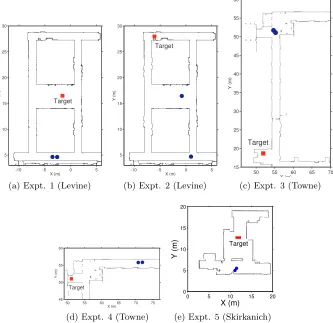
In Experiment 1, we place two robots within 0.5m of each other and put the target in NLOS conditions approximately 16m away. A good control strategy for this experiment will result in the robots moving in complementary directions rather than staying tightly clustered together.

For Experiment 2, we place the robots far away from each other to see if they still move in complementary directions. The separation also tests whether the measurement model consistently combines measurements from different modalities; if the robots follow good trajectories, they will achieve LOS to the target at different times.

(45)

X (m) Y (m) _Target

-10 -5 0 5

5 10 15 20 25 30

(a) Expt. 1 (Levine)

X (m)

Y (m)

Target

-10 -5 0 5

5 10 15 20 25 30

(b) Expt. 2 (Levine)

X (m)

Y (m)

Target

50 55 60 65 70

15 20 25 30 35 40 45 50 55 60

(c) Expt. 3 (Towne)

X (m)

Y (m)

Target

50 55 60 65 70 75 45

50 55 60

(d) Expt. 4 (Towne)

X (m)

Y (m)

Target

0 5 10 15 20

(e) Expt. 5 (Skirkanich)

(46)

wood or metal framing with drywall. Experiments 3 and 4 take place in Towne Building which was built in 1906 – its walls are typically made of brick or concrete.

For Experiment 4, we again place the robots close to each other with the target 20m along a hallway that has a slight bend. The robots and the target do not have geometric LOS, but the wall between them just barely obstructs their view, making it ambiguous whether or not the RF signal will exhibit LOS or NLOS behavior.

In Experiment 5, we examine how the robots move when they are in a more open environment. The robots start next to each other and have more control options to select from than in the first four experiments since they are not constrained to move along a hallway. This experiment takes place in Skirkanich Hall which was completed in 2006 and also features modern construction materials.

Fig. 3.4 shows the starting location of the target and robots for each experiment.

3.2.2 Equipment and Configuration

We use the 3rd generation of the Scarab mobile robot Sect. A.1. The Scarabs are simple differential drive robots equipped with laser scanners for localization and 802.11s wireless mesh cards for communication [82]. The experimental software is developed in C++ and

(47)

X (m)

Y (m)

-10 -5 0 5

5 10 15 20 25

(a) Levine

X (m)

Y (m)

50 55 60 65 70 75 80 85

15 20 25 30 35 40 45 50 55

(b) Towne

X (m)

Y (m)

0 5 10 15 20

(c) Skirkanich

Figure 3.5: Graphs for candidate locations. Delaunay triangles are shown along with their incenters which form the vertices of the graph.

Table 3.2: Measurement Model Parameters. LOS NLOS

α0, β0 2.51 -1.34

α, β 0.20 -0.24

σ2_L, σ2_N 7.00 14.01

distinct choices. In Ch. 4 we develop a theoretical justification for these parameters by proving that mutual information cannot change substantially when the robot’s position change doesn’t change substantially more than the standard deviation of individual range measurements.

(48)

Table 3.3: Computational complexity of control law. (3.3) with nparticles,lrobots, andd

potential locations per robot.

Task Cost

Single Evaluation Θ(n2l) Solving Objective Θ(n2_ldl₎

3.2.3 Results

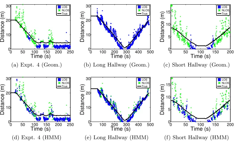
Fig. 3.6 shows the error of the nanoPAN 5375’s measurements as a function of distance. At short distances in LOS conditions the nanoPAN provides consistent measurements with an error larger than 2.0m. In NLOS conditions there is significant variability in both the mean and variance of the measurements as the distance between source and receiver increases. This data helps justify our choice of measurement model as it is clear that LOS and NLOS conditions have different sensor measurement biases and variances.

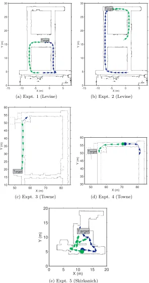
Overall, our approximation of mutual information resulted in good trajectories for the robots. Fig. 3.7 shows that the robots moved to gain complementary measurements; they moved orthogonally to one another when possible, and once they had localized the source, they maintained LOS. Fig. 3.8 shows this process in more detail. Initially, both robots moved away from each other. Next, the robot on the left moved up the vertical hallway, while the other robot moved laterally; an orthogonal movement pattern. Once measurements along the horizontal hallway were no longer helpful due to the symmetry of the distribution, Fig. 3.8b, both robots moved up the vertical hallway, which caused the filter to converge. We stress that these behaviors arose organically from our objective.

Fig. 3.8 also serves as a good example of the types of distributions that typical parametric approaches that assume a unimodal distribution cannot reliably track as there are clearly multiple equally valid hypotheses.

(49)

−10 −5 0 5 10 15 20 25

0 5 10 15 20 25

Distance (m)

Bias (m)

(a) LOS, Levine

−10 −5 0 5 10 15 20 25

5 10 15 20 25

Distance (m)

Bias (m)

(b) NLOS, Levine

−10 −5 0 5 10 15 20 25

0 2 4

Distance (m)

Bias (m)

(c) LOS, Towne

−10 −5 0 5 10 15 20 25

5 10 15 20 25

Distance (m)

Bias (m)

(d) NLOS, Towne

−10 −5 0 5 10 15 20 25

2 4 6 8

Distance (m)

Bias (m)

(e) LOS, Skirkanich

−10 −5 0 5 10 15 20 25

4 6 8

Distance (m)

Bias (m)

(f) NLOS, Skirkanich

Figure 3.6: How geometric LOS and NLOS affects nanoPAN range measurements. The subfigures show standard box-plots with outliers marked as×’s. Each plot contains approx-imately 10,000 data points. NLOS conditions are significantly noisier than LOS conditions with statistics that vary with distance.

Table 3.4: Mean and std. dev. of RMSE of filter’s error over last 30 seconds for each experiment. The error is lower when using an HMM, particularly in Expt. 4.

Expt. 1 Expt. 2 Expt. 3 Expt. 4 Expt. 5

(50)

X (m)

Y (m)

Target

-15 -10 -5 0 5

0 5 10 15 20 25 30

(a) Expt. 1 (Levine)

X (m)

Y (m)

Target

-15 -10 -5 0 5

0 5 10 15 20 25 30

(b) Expt. 2 (Levine)

X (m)

Y (m)

Target

50 60 70 80

10 15 20 25 30 35 40 45 50 55 60

(c) Expt. 3 (Towne)

X (m)

Y (m)

Target

50 60 70 80

30 35 40 45 50 55 60

(d) Expt. 4 (Towne)

X (m)

Y (m)

Target

0 5 10 15 20

(e) Expt. 5 (Skirkanich)

(51)

11.02 sec X (m) Y (m) 26 32 T

−20 −10 0 10

−15 −10 −5 0 5 10 15 20 25

(a)t= 11.02 s

30.14 sec X (m) Y (m) 26 32 T

−20 −10 0 10

−15 −10 −5 0 5 10 15 20 25

(b)t= 30.14 s

112.27 sec

X (m)

Y (m)

26 32 T

−20 −10 0 10

−15 −10 −5 0 5 10 15 20 25

(c)t= 112.27 s

Information-Theoretic Active Perception for Multi-Robot Teams

Acknowledgements

Contents

List of Tables

List of Figures

Chapter 1

Introduction

1.1

Research Problems

1.2

Thesis Overview

Chapter 2

Background and Related Work

2.1

Information Theory

p

(

X

=0)

Entropy (bits)

2.2

Information Based Control for Robotics

2.3

Limited Information Active Perception

2.4

Information Rich Active Perception

Chapter 3

Estimation and Control for

Localizing a Single Static Target

3.1

Technical Approach

3.2

Experiments