On a Characteristic of Data Transmission with Three or
More Priority Levels in Bus Network
M. Ooki*
Dept. of Integrated System Engineering, Computer System Course, Nishinippon Institute of Technology, Japan.
* Corresponding author. Email: [email protected]
Manuscript submitted August 5, 2016; accepted March 14, 2017. doi: 10.17706/ijcce.2017.6.2.137-150
Abstract: This paper presents a characteristic of data transmission in bus network in which each datum has
a priority and the number of priority levels are three or more. In this bus network, each station is connected to a bus through a switching-hub which establishes a link from a sending station to a receiving station. When the receiving station is sending data or receiving data, the link cannot be established and the sending station has to wait a little waiting time (stand-by time). Then, by defining the link probability as a constant, the bus network is analyzed.
Taking note of one of the sending stations with r(r≥3) sending buffers for data with priority, in steady state, a balance equation of the probabilities of the number of waiting data at the ready time of sending is expressed. From the equation, for each priority, probabilities of the number of waiting data, mean of the number of waiting data in the sending buffer and mean waiting time which is the time from the arrival time of a datum at the sending buffer to the beginning time of sending the datum are derived. The calculated values of mean waiting time are illustrated and mean waiting times with priority processing are compared with mean waiting time without priority processing. As a result, the influence of the link probability on data transmission with priority processing is clarified.
Key words: Bus network, priority processing, probability of the number of waiting data, mean of the
number of waiting data, mean waiting time.
1.
Introduction
In bus network which is a primary topology for LAN (Local Area Network), recently, stations are connected to a bus through a switching hub which establishes a link from a sending station to a receiving station. As studies in bus network, the proposal of the dynamic bandwidth allocation [1] for Ethernet PON(Passive Optical Network), the time synchronization on Gb/s Ethernet [2] which is necessary for the wide distributed system and the host configuration mechanism to network in Ethernet and wireless LAN [3] are studied. For application of Ethernet, an application method in industry [4], the performance of industrial Ethernet [5] and the performance of TDMA based network [6] are reported. And, about ad hoc network, impact of mobility [7], [8] are studied.
In bus network with a switching hub, a sending station has to wait for sending when the receiving station is sending or receiving data. I already reported a characteristic of data transmission in bus network under the condition that the link probability is defined as a constant [9], [10].
with priority [14] are reported. I also reported bus network with two priority levels [15]. However, in order to consider a characteristic of bus network with more priority levels, the analysis in the case of two priority levels is not sufficient.
In this paper, a characteristic of data transmission with priority processing in bus network which has three or more priority levels is clarified. Taking note of one of the sending stations which has r(r≥3) sending buffers for data with priority, probabilities of the number of waiting data, mean of the number of waiting data in the sending buffer and mean waiting time from the arrival time at the sending buffer to the beginning time of sending are derived. Furthermore, the calculated values of mean waiting time are illustrated and mean waiting times with priority processing are compared with mean waiting time without priority processing. As a result, the influence of the link probability on data transmission with priority processing is clarified.
2.
Modeling Of Bus Network with Three or More Priority Levels
The bus network shown in Fig. 1 is analyzed.
Fig. 1. Bus network with three or more priority levels.
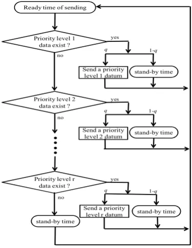
Fig. 2. Flowchart of data transmission.
In the network, each station has r(r≥3) infinite buffers for priority level data, which are called as sending
Switching hub
Stations
Priority level 1 data Priority level 2 data Priority level 3 data
・ ・ Priority level r data
Priority level 1 data Priority level 2 data Priority level 3 data
・ ・ Priority level r data
Priority level 1 data Priority level 2 data Priority level 3 data
・ ・ Priority level r data
Ready time of sending
Priority level 1 data exist ?
stand-by time Send a priority
level 1 datum
1-q
yes
no
q
stand-by time Priority level r
data exist ?
yes
no
1-q q
Send a priority
level r datum stand-by time Priority level 2
data exist ?
stand-by time Send a priority
level 2 datum
yes
no
:
:
Poisson process. Priority level 1 is the highest level and priority level r is the lowest. The arrival ratio for
priority level i (i=1,2,⋯, r) data is i. At the ready time of sending, if priority level 1 data exist in the sending
buffer and a link to a receiving station is established, the station sends the first priority level 1 datum in the sending buffer. If not established, the station has a little waiting time (called as stand-by time). If there is no priority level 1 data, the station checks priority level 2 data. If priority level 2 data exist and the link is established, the station sends the first priority level 2 datum. If not established, the station has stand-by time. If there is no priority level 2 data, the station checks priority level 3 data. The same processing is performed, and finally, if priority level r data exist and the link is established, the station sends the first priority level r datum. If not established, the station has stand-by time. If there is no priority level r data, the station has stand-by time. Defining the link probability as a constant q, the flowchart of data transmission is shown in Fig. 2.
Taking note of one of the sending stations, the sending station is modeled as Fig. 3.
Fig. 3. Model of a sending station.
Transmission time is arbitrary distributed and the distribution function (DF) of the transmission time for each priority level data is denoted by Hi(t) (i=1,2,⋯,r). The stand-by time is arbitrary distributed and the DF of the stand-by time is denoted by Hc(t).
3.
Probability of the Number of Waiting Data
Balance Equation
3.1.
Let Pn1,n2,⋯,nr be the probability that the number of priority level i(i=1,2,⋯,r) waiting data in the sending
buffers is ni at the ready time of sending. In steady state, the following balance equation is obtained.
3
3
1
, , , ,
1 0 0
0 1
3 3 3 0 , ,
1 0 0
0
0
α 1, α , α ,
α , α 1, α , α ,
α
1 2 r
1 2 r 1 2 r
1 2 r
2 r
2 r
2 r
n ' n ' n '
n ',n ' n ' 1 1 1 2 2 2 r r r n ,n n 1
n n n
n '
n ' n '
1 1 2 2 2 r r r ,n n 2
n n n
1 1
P q n ' n t n ' n t n ' n t P dH t
q n ' t n ' n t n ' n t n ' n t P dH t
q n
1
1
1
2 2 1 1 0 ,0,
1
1 1 1 , ,
0 0 0
0
, α , α , α 1,
1 α , α , α ,
r
r r
2 r
1 2 r
2 r
n '
r r r r r , n r
n
n ' n ' n '
2 2 2 r r r n ,n n c
n n n
' t n ' t n ' t n ' n t P dH t
q n ' n t n ' n t n ' n t P dH t
(1)Link probability q→H1(t)
Priority level 1 data
If not exist →Check level 2 data
λ
1
Sending datum
(1-q)→Hc(t)
Sending buffers
λ2
Priority level 1 data
Priority level 2 data
Link probability q→H2(t)
Priority level 2 data
If not exist →Check level 3 data
(1-q)→Hc(t)
Link probability q→ Hr(t)
Priority level r data If not exist→Hc(t)
(1-q)→ Hc(t)
・ ・ ・
λ
r Priority level r data
In equation (1), αi
n t, is the probability that n priority level i data arrive at the sending buffer within time t.
e
λ
λ
α
,
!
it n
i i
t
n t
n
(i=1,2,⋯,r) (2)Here, in order to make analytical procedure plain, let the number of priority levels be 3, i.e. r=3.
Taking
2 3
0 0 0
1 n ' n ' n '
after multiplying 1 2 31 2 3
n n' n' '
x x x in both sides of equation (1) under r=3 and
transforming into a generating function form, the following equation is obtained.
2 3 1 *2 2 3 2
2
*
3 3 3
3
*
, ,
1
1
[
,
1
1
1
1
1
1 ]
1 1 * * c 1 * c *c 0,0,0 c
G x x x
q
H
z
q H z
x
q
G x x
H
z
q H z
x
q
G x
H
z
q H z
P
H z
x
(3)where Hi*(z) (i=1,2,3) and Hc*(z) are the Laplace-Stieltjes Transformation(LST) of Hi(t) and Hc(t), respectively, and z λ 11
x1
+λ 12
x2
+λ 13
x3
.The generating functions of the probabilities of the number of waiting data are defined as follows.
22
, ,
1 0 0
3 1
1 2 3
1 3
n
n n
1 1 2 3 n n n 1 2 3
n n n
G x ,x ,x
P
x x x
(4a)
22
0, , 2
1 0
,
3 2 3 3 n n2 2 3 n n 3
n n
G x x
P
x
x
(4b)
0,0,1
3 3 3
n
3 3 n 3
n
G x
P
x
(4c)Probabilities of the Number of Waiting Data
3.2.
When x1x2x31 in equation (3), the following equations are obtained.
1 1 1 1
1 1 1
λ
1
λ
1,1,1
λ
1
λ
1,1
λ
1
λ
1
λ
0
1 c 1 2 c 2
3 c 3 c 0,0,0
q q h
q
h
G
q h
q
h G
q h
q
h G
h P
(5a)
2 2 2 2
2 2 2
λ
1
λ
1,1,1
λ
1
λ
1,1
λ
1
λ
1 +λ
0
1 c 1 2 c 2
3 c 3 c 0,0,0
q h
q
h
G
q q h
q
h G
q h
q
h G
h P
3 3 3 3
3 3 3
λ
1
λ
1,1,1
λ
1
λ
1,1
λ
1
λ
1 +λ
0
1 c 1 2 c 2
3 c 3 c 0,0,0
q h
q
h
G
q h
q
h G
q q h
q
h G
h P
(5c)In equation (5a), (5b) and (5c), hi and hc are means of Hi(t) and Hc(t), respectively. Because the sum of all probabilities is equal to 1, equation (6) is obtained.
1,1,1
1,1
1 11 2 3 0,0,0
G G G P (6) From equation (5a), (5b), (5c) and (6), the following probabilities are derived.
11 2 3 1 2 3
λ
1,1,1
{1 (λ
λ
λ
) (λ
λ
λ
)
}
c 1
1 2 3 c
h
G
q
h
h
h
h
(7a)
21 2 3 1 2 3
λ
1,1
{1 (λ
λ
λ
) (λ
λ
λ ) }
c 2
1 2 3 c
h
G
q
h
h
h
h
(7b)
31 2 3 1 2 3
λ
1
{1 (λ
λ
λ
) (λ
λ
λ ) }
c 3
1 2 3 c
h
G
q
h
h
h
h
(7c),0
1
(1,1,1)
(1,1)
(1)
0,0 1 2 3
P
G
G
G
(7d)
1,1,1
1
G is the probability that the number of priority level 1 waiting data is one or more at the ready time of sending. G2
1,1 is the probability that the number of priority level 1 waiting data is 0 and priority level 2 data is one or more. G3
1 is the probability that the number of priority level 1 and level 2 waiting data is 0 and priority level 3 data is one or more. P0,0,0 is the probability that there is no waiting data.4.
Mean of the Number of Waiting Data
Priority Level 1
4.1.
From equation (3),
11
,1,1 |
1 1 x
1
d G x
dx which is mean of the number of priority level 1 waiting data in the
sending buffer can be derived.
From equation (3), G x1
1,1,1
is expressed by equation (8), (9a) and (9b).
1
1A ,1,1
B
1 1 1
1 x G x
x
(8)
1
3 3
0 0 0
A
(1,1)
+(1 q)
1
(1)
+(1 q)
1
+P
1
* *
1 2 2 1 c 1
* *
1 c 1
*
c 1
x
G
qH z
H z
G
qH z
H z
H z
,,
1
B
1
*1
*1 1 1 c 1
1
q
x
H
z
q H z
x
(9b)where
z
1
λ 1
1
x
1
.When
x
1
1
after differentiating equation (8), the following equation is obtained
1
1 1 1 1
1 2
1
A 1 B 1
A 1 B 1
,1 |
2 B 1
1 1 x
1
"
'
'
"
d
G x
dx
'
(10)where
'
1 1 1
1 1 1
A 1
(1,1){ λ
(1
)λ }
+ (1){ λ
(1
)λ }+
λ
2 2 c
3 3 c 0,0,0 c
G
q h
q
h
G
q h
q
h
P
h
(11a)
'
1 1 1
B 1
q q h
λ
1
1 q λ
h
c (11b)and
2 21 1 1
2 2 2
1 1 1
A 1
(1,1){ λ
+(1- )λ
}
(1){ λ
+(1- )λ
}+
λ
'' (2) (2)
2 2 c
(2) (2) (2)
3 3 c 0,0,0 c
G
q h
q
h
G
q h
q
h
P
h
(12a)
2
21 1 1 1
B 1
2
2 λ
λ
(2)1 q λ
(2)1 1 c
"
q
q h
q h
h
(12b)(2) i
h
andh
c 2 are the second moments of the DFs of Hi(t) and Hc(t), respectively.Priority Level 2
4.2.
Using
x
1
1( , )
x x
2 3 which satisfies that the denominator of equation (3) is equal to 0, the following equation is obtained.
3
2 2
1
{
1
1}
1
,
1
1
* * *
3 3 c 0,0,0 c?
3 3
* *
2 c
2
G x
qH
z
q H z
P
z
H z
x
G x x
q
H
q H z
x
(13)where
z
λ 1
1
1
x x
2,
3
+λ 1
2
x
2
+λ 1
3
x
3
.and
1
x x
2,
3
satisfies the following equation.
1 1
1
1
0
( , )
* *
c
2 3
q
H
q H z
x
x
z
From equation (13),
2 2 1 2 ,1 | 2 x d G xdx which is mean of the number of priority level 2 waiting data in the
case that the number of priority level 1 waiting data is 0 can be derived. From equation (13), G x2
2,1
is expressed by equation (15), (16a) and (16b).
2
2 2 2 A ,1 B 2 2 x G x x (15)
2 2 2 0,0,0 2
A
(1){
*(1
)
*1}
*1
2 3 3
z
c cx
G
qH
q H z
P
H
z
(16a)
2
2 2
B
1
*1
*2 2 c
2
z
H
z
q
x
q H
x
(16b)where
z
2
λ 1
1
1
x
2,1 +λ 1
2
x
2
.When
x
2
1
after differentiating equation (15), the following equation is obtained.
2 2 2 2
1 2
2
A
1 B 1
A 1 B
1
,1 |
2 B 1
2
2 2 x
2
"
'
'
"
d
G x
dx
'
(17)
2
A 1
'(1){
(1
)
}
3
z' h
20 3q
20 c 0,0,0 20 cG
q
z' h
P
z'
h
(18a)
2
B
'1
20 2(1
)
2 c0
q qz' h
q z' h
(18b)where 1 2 2 20 x
z'
z'
and
22
2 3
2
)
(1
)
)
A
1
(1){ (
(
(
1
)
}
{
(
)
?
}
20 20 3 20
20 c 20 20 c
'' (2) (2)
3 c
(2)
0,0,0 c
G
q
z'
h
q
z" h
q z'
h
z" h
z'
z"
q
P
h
h
(19a)
2 2 2 2 2
2
B
1
2
2
(
(1
)(
(
)
)
)
1
20 20 (2) 20
20 20
(2)
c c
z'
z'
z"
"
q
q
h
q
h
q
h
q
z'
h
q "
z h
(19b)where 1 2 2 20 x
z"
z"
.On the other hand, from
z
2
λ 1
1
x
2
+λ 1
2
x
2
.and equation (14) under x31, the following equations are obtained.
2 2 10 1 1
(1
)
(1
)
1 c 1 cq h
q
h
'
q q h
q
h
1 10 2
20
z'
'
(20b)
2 (2) (2)10 1
2 2
10
1 1
2
0
)
)
2
2
(
(
(
(1
)
)
(2)
1 20 c 20 1 20
1 c
20 c
q '
q ' h
h
qh
h
"
q q
z'
z'
z'
q
h
q
z'
h
(20c)
1 10
20
"
"
z
(20d)From these equations,
z'
20 andz"
20 can be calculated.Priority Level 3
4.3.
Using x2
2( )x3 which satisfies that the denominator of equation (13) is equal to 0, the followingequation is obtained.
*
3 3
1
1
1
0,0,0 c
3 3
* *
c
P
H z
G x
q
H z
q H z
x
(21)where
z
λ 1
1
1
2( ),
x
3x
3
+λ {1
2
2( )}+λ 1
x
3 3
x
3
.and 1
2( ),x3 x3
and 2( )x3 satisfy the following equations.
1 2 3
1
1
0
( ( ), )
* *
1 c
3
z
q
H z
H
q
x x
(22)
2
1
1
0
( )
* *
2 c
3
q
H
q
x
z
H
z
(23)From equation (21),
| 13 3 3 x 3
d G x
dx which is mean of the number of priority level 2 waiting data in the
case that the number of priority level 1 and level 2 waiting data is 0 can be derived. From equation (21),
3 3G x is expressed by equation (24), (25a) and (25b).
3
3
A
B
3
3 3
3
x
G x
x
(24)
3 3
A
*1
0,0,0? c
x
P
H z
(25a)
3
B
1
*1
*3 3
z
cq
z
x
H
q H
x
When
x
3
1
after differentiating equation (21), the following equation is obtained.
3 3 3 3
1 2
3
A
1 B 1
A 1 B 1
|
2 B 1
3
3 3 x
3
"
'
'
"
d
G x
dx
'
(26)
3
A 1
'0,0,0 0 c
P
z'
h
(27a)
33
B
'1
(
1
)
0 c0
z' h
'
q
q
h
q
z
(27b)where
1
3 x 0
z'
z'
.and
23
A 1
''{
(
0)
(2)}
0 0 0, ,
z
c 0 cP
'
h
z"
h
(28a)
2 3
2
B 1
2
2
)
)
(
(1
)(
(1
)
(2)
3 3 3
(2) c
0 0 0
0 0 c
z'
z'
z"
"
q
q h
q
h
q
h
z'
z" h
q
h
q
(28b)where
1
3 x 0
z"
z"
.On the other hand,
1 1 2 3
λ 1
2( ),
3 3+λ {1
2( )}+λ 1
3 3z
x
x
x
x
and equation (22), (23),
'
20,
'
130,
z'
0 and
"
20,
"
130,
z"
0 can be derived.Here,
'
20
' x
2( )
3 x31,
'
130
'
1( ( ) )
2x x
3 3 x31,
z'
0
z'
x31,20 2
( )
3 x3 1,
130 1( ( ) )
2 3 3 x3 1,
0 x3 1"
" x
"
"
x x
z"
z"
.5.
Mean Waiting Time
Priority Level 1
5.1.
The probability that the number of priority level 1 waiting data at the end of sending data is
n'
1 isdenoted by
1
1
R
n ', and then the following equation is obtained.
1
1 2
' 1
1 1
1 0 0
0
1
α
1,
d
1,1,1
1 1 2 3
3 n
1n ' 1 n ,n ,n 1
n n n
1
R
n ' n
t
P
H t
G
Taking
1' 0
n
after multiplying 11
' n
x
in both sides in equation (29), and transforming into equation of theGF, equation (30) is obtained.
1
1
1
1
,1,1
1,1,1
1
*
R 1 1 1
1
G
x
G x
H
z
x G
(30)where
0
1
1 1
1
n '
R 1 1n ' 1
n '
G
x
R
x
.On the other hand, the probability that the number of priority level 1 arrival data during waiting time and sending time for priority level 1 data is
n '
1 is equal to1 1n '
R
, so that the following equation is obtained.
1 0
α
, d
1
1n ' 1 1 1
R
n ' t W t
H t
(31)where
W t
1
is the DF of waiting time for priority level 1 data and
is a convolution operator.Taking
1' 0
n
after multiplying 11
' n
x
in both sides of equation (31) and transforming into equation of theGF, equation (32) is derived.
*
*
R1 1 1 1 1 1
G
x
W
z
H
z
(32)where *
1 1
W
z
is the LST ofW t
1
.From equation (30) and (32), *
1
W
z
is obtained as follows.
1
1
1
,1,1
1,1,1
*
1 1
1 1
W
z
G x
x G
(33)When
z
1
0
after differentiating equation (33) byz
1, the left side of equation is obtained as follows.
0
d
d
1*
1 1
z 1
1
W
z
w
z
∣
(34a)where
w
1 is mean ofW t
1
.On the other hand, the right side is obtained as follows.
0
1
1
,1,1
d
1
d
,1,1
1,1,1
d
1,1,1
1λ
1,1,1 d
11 1
z 1 1 x 1
1 1 1 1 1
G x
G x
G
z x G
G
x
From equation (34a) and (34b), mean waiting time for priority level 1 data
w
1 is obtained.
1
1
1
d
,1,1
1,1,1
λ
1,1,1 d
11 1 1 x 1
1 1
w
G x
G
G
x
|
(35)
1,1,1
1G
andd
,1,1
1d
1 1 x11
G x
x
|
have been already derived, so that mean waiting timew
1 can becalculated.
Priority Level2 and Priority level 3
5.2.
Similar to priority level 1, mean waiting times for priority level 2 and level 3 are obtained as follows.
1
2
1
d
,1
1,1
λ
1,1 d
22 2 2 x 2
2 2
w
G x
G
G
x
|
(36)
1
3
1
d
1
λ
1 d
33 3 3 x 3
3 3
w
G x
G
G
x
|
(37)
2
1,1
G
,d
,1
1d
2 2 x2 2G x
x
|
,G
3
1
and
1d
d
3 3 x3 3G x
x
|
have been already derived, so that meanwaiting times
w
2 andw
3 can be calculated.Numerical Examples
5.3.
Fig. 4 shows a relation between arrival ratio
λ
1 and mean waiting timesw
1 ,w
2 andw
3 in the case of1 2 3
λ
λ
λ
, q=0.1, 0.5, 0.9,h
1=h
2=h
3=5,h
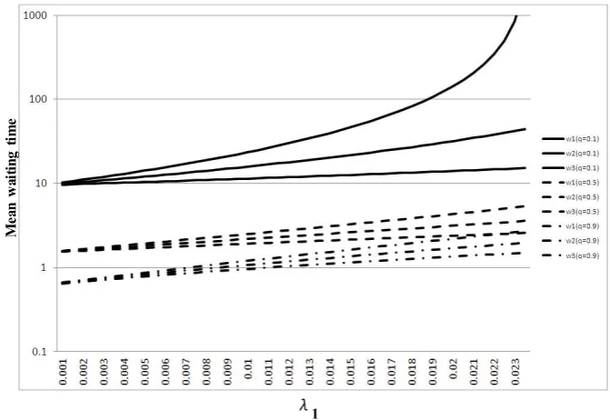
c =1 and Hi(t) and Hc(t) obey uniform distributions.Fig. 4. Mean waiting timew1 , w2 and w3 (h1=h2=h3=5, hc=1, λ1 λ2 λ3, uniform distribution).
M
ea
n
w
ai
tin
g
ti
m
e
λ
Fig. 5. Mean waiting time w1 , w2 and w3 (h1=h2=h3=5, hc=1, λ1 λ2 λ3, exponential distribution).
In Fig. 4, solid lines, dashed lines and chain lines are mean waiting times in the case of q=0.1, 0.5 and 0.9, respectively. In the same lines, the lower line is mean waiting time
w
1 , the middle line isw
2 and theupper line is
w
3 . It is confirmed that the mean waiting time becomes long as the link probability qbecomes low and as the arrival ratio
λ
1 becomes high. In the case of q=0.1, mean waiting timew
3becomes infinite when
λ
1 is over 0.023. This means that when q=0.1 andλ
1 is over 0.023, the sending buffer for priority level 3 is overflow because there are more arrival data than sending data.In the case thatHi(t) and Hc(t) obey exponential distributions, mean waiting times are shown in Fig. 5. Comparing Fig. 5 to Fig. 4, mean waiting times become longer, but Fig. 5 shows similar tendency.
Next, a comparison with mean waiting times in the case of q=0.5,
λ
1
λ
2
λ
3 and mean waiting time without priority processing is shown in Fig. 6.M
ea
n
w
ai
ti
ng
ti
m
e
λ
1
M
ea
n
w
ai
tin
g
ti
m
e
λ
In Fig. 6, bold solid line is mean waiting time without priority processing and thin solid line, dashed line and chain line are mean waiting time
w
1 ,w
2 andw
3 with priority processing in the case of q=0.5,h
1=2
h
=h
3=5,h
c =1, λ1λ2λ3.It is confirmed that mean waiting time
w
1 ,w
2 are shorter, but mean waiting timew
3 is longer than mean waiting time without priority processing. As arrival ratio becomes high, differences of mean waiting times with priority processing and mean waiting time without priority processing becomes long. On the basis of mean waiting time without priority processing, the ratios of difference of mean waiting times are -44.1% inw
1 , -22.1% inw
2 and 66.1% inw
3 on the average.6.
Conclusion
In this paper, a characteristic of data transmission with three or more priority levels in bus network is clarified. In the analysis, taking note of one station, the link probability that the link from the station to a receiving station can be established is defined as a constant. And then, for each priority, the probabilities of the number of waiting data, the mean of the number of waiting data and the mean waiting times are derived. For the analysis of lower priority levels, roots of the denominator of generating functions are used.
In the analysis, at first, the balance equation with arbitrary priority levels is expressed, but the analysis is performed for three priority levels. As for the analysis for more than three priority levels, the analytical procedure of this paper can be used. But, the number of simultaneous equations increases as the number of priority levels increases.
According to the analysis result, some numerical examples are illustrated, and then the influences of the link probability and the arrival ratio of data on the characteristics of data transmission are clarified. Furthermore, the effect of priority processing is confirmed by comparing with mean waiting time with priority processing and that without priority processing.
The characteristic of data transmission with priority processing in this paper is a base of considering efficiency of bus network.
The following considerations remain for further study: (1) Analyzing the bus network with other priority processing.
(2) Clarifying a relation between the link probability and the buffer size of a receiving station.
References
[1] Luo, Y., & Ansari, N. (2005). Dynamic upstream bandwidth allocation over Ethernet PONs. IEEE Int.
Conf. Commun., 2005(3), 1853-1857.
[2] Yamada, Y., Ohta, S., & Uematsu, H. (2006). Hardware-based precise time synchronization on Gb/s Ethernet enhanced with preemptive priority. IEICE Trans. Commun., E89-B(3), 683-689.
[3] Huang, T., & Chu, K. (2011). Networking without dynamic host configuration protocol server in Ethernet and wireless local area network. J. Netw. Comput. Appl., 34(6), 2027-2041.
[4] Decotignie, J. (2005). Ethernet-based real-time and Industrial Communications. Proceedings of IEEE,
93(6), 1102-1117.
[5] Jaspernette, J., Schumacher, M., & Weber, K. (2007). Limits of increasing the performance of industrial protocols. Proceedings of IEEE Int. Conf. Emerge. Tecnol. Fact. Autom., 12(1), 17-24.
[6] Otsuki, N., & Sugiyama, T., (2012). Implementation of a TDMA based wireless network coding prototype system with Ethernet frame aggregation. IEICE Trans. Commun., E95-B(12), 3752-3759.
2003(2), 825-835.
[8] Hara, T., (2010). Quantifying impact of mobility on data availability in mobile Ad Hoc networks. IEEE
Trans. Mob. Comput., 9(2), 241-258.
[9] Ooki, M. (2014). On a characteristic of data transmission in bus network. J. of Advances in Computer Networks, 2(2), 120-124.
[10]Ooki, M. (2014). Simulation for data transmission in bus network. Memoirs of Nishinippon Institute of Technology, 44, 39-44.
[11]Shengxiang, L., Zichun, L., Minglei, F., Zhijun, Z., & Wei, F. (2011). MAC protocol with dynamic priority adjustment for light trail network. Proceedings SPIE, 7989, 798914.1-798914.11.
[12]Vasiliadis, D., Rizos, G., & Vassilakis, C. (2013). Modelling and performance study of finite-buffered blocking multistage interconnection networks supporting natively 2-class priority routing traffic. J. Net. Comput. Appl., 36(2), 723-737.
[13]Cheng-Min, L. (2010). Analysis and modeling of priority inversion scheme for starvation free controller area networks. IEICE Trans. Inf. Syst., E93-D(6), 1504-1511.
[14]Khabazian, M., Aiessa, S., & Mehmet-Ali, M. (2011). Performance modeling of message dissemination in vehicular Ad Hoc network with priority. IEEE J. Sel. Areas Commun., 29(1), 61-71.
[15]Ooki, M. (2015). On a characteristic of data transmission with priority processing in bus network. J. of Advances in Computer Networks, 3(2), 87-92.
M. Ooki was born at Fukuoka in Japan on January 27 in 1953. He graduated from Doctoral
degree course in Kyushu Institute of Technology graduate school in 1992 (doctor of engineering). His major field is communication network system.
He is a Professor of Nishinippon Institute of Technology (Aratsu 1-11, Kanda-machi, Miyako-gun, Fukuoka 800-0394 Japan).