Determining Optimal Tolling Rates for Border Regions Using Dynamic Modeling Methods

(1)

American Journal of Traffic and Transportation Engineering

2019; 4(4): 118-131

http://www.sciencepublishinggroup.com/j/ajtte doi: 10.11648/j.ajtte.20190404.12

ISSN: 2578-8582 (Print); ISSN: 2578-8604 (Online)

Determining Optimal Tolling Rates for Border Regions

Using Dynamic Modeling Methods

Jeffrey Shelton

1, *

, Peter Martin

2 1

Multi-Resolution Modeling, Texas A&M Transportation Institute, El Paso, USA 2

Department of Civil Engineering, New Mexico State University, Las Cruces, USA

Email address:

*

Corresponding Author

To cite this article:

Jeffrey Shelton, Peter Martin. Determining Optimal Tolling Rates for Border Regions Using Dynamic Modeling Methods. American Journal of Traffic and Transportation Engineering. Vol. 4, No. 4, 2019, pp. 118-131. doi: 10.11648/j.ajtte.20190404.12

Received: May 21, 2019; Accepted: July 23, 2019; Published: August 14, 2019

Abstract:

Many toll facilities have been faced with traffic shortfalls due to inaccurate and over-forecasted toll revenue projections. Therefore calculating optimal toll rates can be a difficult process. Toll rates are often set to reflect the revenue needed to pay back bonds issued to finance the roadway. This research provides an alternative approach to calculating toll rates where revenue can be maximized while still considering the socio-demographics of the region. Several different approaches used in the border region were explored and compared to field data on an existing toll facility in El Paso, Texas. An innovative simulation-based modeling approach was used to test both static and dynamic pricing algorithms. Static tolling results showed optimal toll rates of $0.14/mile and $0.08/mile for Border Highway West in the westbound and eastbound directions respectively. The Cesar Chavez Highway has optimal toll rates of $0.12 and $0.10/mile in the west and eastbound directions. The dynamic tolling approach showed a max toll rate of $1.56/mile for Cesar Chavez Highway (westbound) during the morning peak period and then incrementally decreased to the minimum toll rate. However, the eastbound direction never increased above the minimum toll rate of $0.08 mile. Border Highway West never increased above the minimum toll rate in either direction. The dynamic tolling algorithm prediction is more representative of the optimal tolling rates for the border region-with the exception of Cesar Chavez Highway westbound.

Keywords: Dynamic Traffic Assignment, Toll Revenue Forecasting, Optimal Toll Rates, Value of Time

1. Introduction

Increasing traffic congestion is a growing problem for large urban areas. Throughout the United States, traditional funding sources for transportation projects are becoming less able to meet the growing demand for highway infrastructure. State departments of transportation are relying more on alternative methods, such as toll roads, to finance new highway projects. Toll facilities must be able to generate sufficient revenue from operations to cover debt obligations and maintenance costs to be financially viable investments. States mainly located in the North and East began to build state tolls roads on their primary long-distance travel corridors with the goal of collecting revenue to build, improve, and maintain their roadways [1]. In the United Kingdom, the M6 toll road was the first tolled motorway designed to alleviate traffic congestion around

Birmingham and was built under a public-private partnership [2].

(2)

American Journal of Traffic and Transportation Engineering 2019; 4(4): 118-131 119

(only 5 out of 105) analyzed by Bain reflected circumstances under which toll revenues had been under predicted by more than 25 percent [4].

When determining toll rates, the value of time (VoT) is a critical component in revenue forecasting. VoT is the governing factor used in forecast models and can influence the amount of traffic using the tolled facilities. This paper determines optimal toll rates for a border region where socio-demographics are the driving influence of daily toll road usage. Optimal toll rates in this context is defined as the maximum toll rate to charge that relates to a corresponding VoT of the region—in this case study, a border region.

We analyzed several different approaches to derive the VoT, using El Paso, Texas as a case study. A simulation-based modeling approach is used to analyze static and dynamic tolling algorithms. The next section outlines a review of toll revenue forecasting examples in the United States and Europe, followed by the different approaches used in El Paso to derive a VoT for the border region. The last section uses a case study in El Paso, Texas that compares two different tolling algorithms.

2. Literature Review

2.1. Toll Revenue Forecasting

The premise of the long range forecasting is rooted in federal regulation originally required by the Intermodal Surface Transportation Efficiency Act of 1991. All transportation acts since that time have continued the requirement for a financial plan. Currently, Title 23 of the United States Code, Section 134 requires a Metropolitan Planning Organization Long-Range Transportation Plan (LRTP) to contain a financial plan that demonstrates how the adopted LRTP can be implemented [5].

In terms of toll revenue forecasting, the number of toll transactions is critical to the feasibility of toll road projects. However, toll road traffic in many countries has failed to reproduce forecasted traffic levels and the associated revenue generated to successfully maintain, operate, and repay financial obligations [6]. If actual traffic is lower than the forecasted amount, the toll road will incur difficulties in delivering the expected returns to its shareholders. Experts have suggested many reasons for this discrepancy including strategic misrepresentation, errors in land-use forecasts, and errors in the specific assumptions and parameters underlying the traffic assignment models used to develop traffic forecasts. Hence, traffic demand forecasting is a critical input into the financial and economic appraisal of toll road projects [7].

In recent years, there is increased incidence of actual traffic falling short of the traffic forecasts, often as much as 50 percent [5]. Flyvbjerg et al. (2006) collected data on real and predicted traffic numbers during the first year of operation, covering 183 road projects around the world. They found that approximately half of those road projects have a forecasting error of more and ± 20 percent, and 25 percent of them have an error of ± 40 percent [8].

The National Cooperative Highway Research Programs (NCHRP) published a synthesis of highway practice looking specifically at revenue studies and the associated demand. NCHRP reported toll revenues as a percentage of those forecasted in 26 U. S. toll facilities over their first five years of operation. Actual toll revenue was 30–40 percent below the predicted values. In total, 104 separate studies were analyzed; only 13 were within ± 10 percent and one third fell within ± 25 percent of predicted revenues [9].

Based on the previous discussion, it can be concluded that traffic demand risk could be mainly attributed to the uncertainty associated with the model assumptions and inputs. However, it is not easy to obtain perfect data representing the model variables. In 2007, Vassallo published the results from a small sample study of toll road forecasts in Spain. Vassallo suggests that opening year forecasts are the most difficult to make. Even though traffic forecasts improved after year 1, there was a clear bias toward the overestimation of traffic [10]. Demand estimation is a complex process involving multiple interdependent variables that affect the demand internally. In toll revenue forecasting, it is the production of complex interactions between travel time savings, VoT, and tolls [11].

2.2. Toll Forecasting Models

In order to predict the forecasted amount of traffic needed to meet revenue projections, a regional traffic forecasting tool (model) is needed. The vast majority of traffic forecasting packages use a traditional four-step macroscopic planning model (also known as travel demand models [TDMs]). The four-step process includes trip generation (how many trips are generated), trip distribution (where do trips go), mode choice (what travel mode is being used for each trip), and trip assignment (what is the route of each trip). In TDMs, trip assignment (route choice) is determined by evaluating and comparing a generalized cost across several alternative routes [12]. A generalized cost consists of travel time and any associated monetary costs (tolls). The generalized cost in its simplistic form can be notated as:

= + (1)

where:

=

= Travel time for vehicle type m on route p

= ! " ℎ $% % = & " " ℎ $% %

(3)

120 Jeffrey Shelton and Peter Martin: Determining Optimal Tolling Rates for Border Regions Using Dynamic Modeling Methods

incorrect use of the VoT may cause serious distortion of investment priorities and potentially an overestimation of forecasted traffic and associated toll revenue [13].

Macroscopic TDMs have limitations when forecasting traffic in general. The trip assignment in TDMs is static in nature, so there is no time-varying properties of traffic flow [14]. They cannot analyze traffic congestion as a concept of time (i.e., queuing on roadways) nor can they analyze congestive-responsive tolling. In addition, TDMs have limitations in terms of realism of actual traffic on a roadway. In a TDM, inflow to a link is always equal to outflow: the travel time simply increases as the inflow and outflow (volume) increases. The volume on a link may increase indefinitely as represented by a volume-to-capacity (v/c) ratio >1. Since the link volume does not conform to the traffic flow limit that results from the physical characteristics of the roadway, the assigned link volume can exceed the physical capacity (in vehicles/hour). The drawback of TDMs using a v/c ratio is that it does not directly correlate traffic flow theory properties—more specifically speed, density, flow, or queuing [15]. In other words, you cannot stack cars on a freeway—but TDMs are still the preferred method for traffic and toll revenue forecasting.

A new approach to traffic forecasting uses a mesoscopic regional model. The mesoscopic model replaces the static trip assignment found in TDMs with a dynamic traffic assignment (DTA) algorithm. Mesoscopic models attempt the rendering of macroscopic traffic flow properties such as speed, density, and flow, but now describes greater decision rules of the individual traveler such as time-dependent route decisions and departure time. In other words, decision rules have now been updated from an aggregated context to a time-dependent context with time-varying conditional changes such as speed, density, and flow. However, rather than representing traffic in the averaged context of macroscopic models of flow, the mesoscopic model explicitly simulates individual vehicles. To be more precise, the mesoscopic model captures individual driver conditions from a lesser time resolution from fractions of a second to fractions of a minute, typically a tenth of a minute, or every six seconds [16].

Zhang et al used an adaptive toll optimization methodology and developed improved calibration algorithms utilizing DynaMIT—a mesoscopic multi-modal multi-data source driven, simulation-based short-term traffic prediction [17]. Zhang et al. applied this methodology in the context of managed lanes where decisions on toll usage is taken in real-time every five minutes. They state that the effectiveness of the toll optimization algorithm can only be tested when the demand and travel behavior are represented accurately. The toll algorithm developed is fully integrated with DynaMIT to find the best toll that provides maximum revenue subject to network conditions given by tolling regulations [18].

Wang et al. developed real-time optimization framework where the toll optimization is also integrated with DynaMIT, so the tolls are optimized based on predicted traffic conditions. DynaMIT embeds several modules including demand simulation, supply simulation, and online calibration. The toll

optimization module is in complete interaction with DynaMIT such that the optimized toll is decided with several iterations between the two rather that a single feedback function. There are two main formulations—the first maximizes revenue and the second considers the traffic conditions on managed lanes while maximizing revenue. Their methodology demonstrates that the framework generates consistent results such that as the demand increases or the willingness to pay (i.e. VoT) is higher, the optimized tolls are higher [19].

Li et al. introduces an agent-based dynamic feedback-control toll pricing strategy that accounts for the trip purpose, travel time reliability, departure time choice and income level such that the toll revenue is maximized while maintaining a minimum desired level of service on the managed lanes. They used an agent-based model to simulate drivers’ learning process based on their previous commuting experience. The study shows that how drivers’ heterogeneity in VoT, and value of reliability for each trip purpose will influence route decisions and thus affect the optimal toll rates using a case study on Interstate 95 express lanes [20].

In summary, a mesoscopic resolution model is a suitable model to simulate the time-varying conditions (e.g., speed, density, and flow) of a large-scale model, yet is efficient in depicting the behavior of the individual driver in adapting speed/density conditions surrounding individual vehicles. Because of the effective representation of traffic dynamics in the framework of large-scale applications, mesoscopic resolution simulation models have been a fundamental part of DTA modeling in recent years, but this type of toll revenue forecasting is mostly limited to university-based research.

3. Value of Time—Existing Approach in

Border Region

After decades of research, VoT calculations remain incompletely understood, so further theoretical and empirical studies are needed. Research has revealed the inconsistencies between the willingness to pay and travel time savings. The value of travel time savings is a critical parameter in the evaluation of toll roads. Travel time savings remains the dominating user benefit associated with improvements to road infrastructure. It is widely accepted as a major influence on traffic and revenue predictions where tolls are assessed by actual and potential users relative to the savings in travel time [21].

The current practice of forecasting the demand for new toll roads typically assumes that car users are prepared to pay a toll for a shorter journey, and they will keep doing so as long as the toll cost is not higher than their current value of travel time savings [22]. One of the main problems of this approach is how road users perceive their VoT. These are critical elements when evaluating road pricing transportation projects.

(4)

methods to estimate the VoT, but a more robust method is needed to help improve the forecasted reliability when evaluating toll lanes, high occupancy vehicle, or incentive clauses during roadway construction. This research analyzes existing approaches used to derive the VoT using previous case studies in Texas. The goal of this research is to develop a more robust methodology that will help improve the reliability of forecasted results when evaluating future road pricing projects, managed lanes, and road user cost calculations.

3.1. Consumer Price Index

A literature review from existing practices in Texas was used

to derive the VoT for the El Paso region. The Texas Department of Transportation (TxDOT) was using a VoT set at $21.73 for passenger cars and $31.71 per hour for trucks (2014 rates). These values were set by the state for road user cost calculations used in A+B bidding and incentive/disincentives milestones, final project completion, and lane rentals [23]. However, the TxDOT VoT was an aggregated average across the entire state of Texas and not indicative of the lower median income in El Paso compared to other large urban areas within the state. The median income for the five largest cities in Texas are outlined in Figure 1 and include Dallas, San Antonio, Austin, Houston, and El Paso.

Figure 1. Median Income – Texas Urban Areas.

The El Paso median income of $40,179 is approximately 24 percent lower than the aggregated statewide average for Texas, which is $53,096. Therefore, the base 2014 VoT for El Paso was reduced by the same percentage, yielding a monetary value of $16.48 for cars using 2014 dollars. Using the Consumer Price Index (CPI), an annual escalation rate was used to determine the base VoT for passenger cars. The CPI from 2001 to 2016 averaged a 2.06 percent increase over the last 15 years. A future value was calculated using the nominal future sum of worth at a given time assuming the calculated annual CPI growth rate:

' = ( ∗ 1 + +₍₂₎ where:

' = ' " ( = ( "

= , - ℎ .(,

= / ℎ %

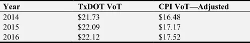
Table 1 compares the VoTs used by TxDOT to the

CPI—adjusted value for the past three years. The VOTs obtained represent adjusted rates for all trips in the El Paso region (forecasted to 2016 dollars), regardless of trip purpose.

Table 1. VoT Comparison—TxDOT versus CPI.

Year TxDOT VoT CPI VoT—Adjusted

2014 $21.73 $16.48

2015 $22.09 $17.17

2016 $22.12 $17.52

3.2. Weighted Trip Purpose—VoT

Additional literature review shows the VoT has a direct correlation to trip purpose (e.g., home-work, work-home). The TxDOT 2016 road user cost VoT for cars ($22.12) was weighted based on the El Paso Metropolitan Planning Organization (MPO) TDM diurnal factors1 to determine the percentage of home-work and work-home versus all other trip purposes (e.g., home-other, other-home, non-home based, external local, through and non-home based external local). Trip purposes were weighted based on the percentage of total trips distributed throughout the day. Figure 2 shows the

(5)

122 Jeffrey Shelton and Peter Martin: Determining Optimal Tolling Rates for Border Regions Using Dynamic Modeling Methods

temporal pattern of home-work and work-home trips. During the morning peak period, home-work trips account for 68 percent of all trips made in a 24-hour period while during the afternoon peak, work-home trips account for 63 percent of all associated trips. The VoT for the region was calculated using:

=

∑425612 32

∑425612 (3)

where:

=

78= ( - % % %

98= , " % % %

Figure 2. Home-Work Related Trips.

Since leisure trips (e.g., non-home-based trips) do not warrant the same VoT as work-related trips, the car VoT was discounted in half for all other trip purposes [24]. Therefore, a VoT of $22.12 for work-related trips was used, while non-work-related trips

were discounted by 50 percent to $11.06. Using a weighted average approach, the home-work and work-home trips account for 23 percent of all trips in the El Paso region. Using equation 2, the VoT for El Paso was calculated to be $13.61 (2016 dollars).

Figure 3. Total Annual Person Trips for Texas [26].

3.3. Demographics

A socio-demographic approach was used to calculate the VoT

(6)

relates to driving (16–70 were considered working age), and population per zone. The average wage rate per zone was calculated based on a typical 2080 hours of work in a calendar year. The median wage per zone was then extracted and weighted against the entire population. The National Household Travel Survey (NHTS) was also used to obtain the percentages of all trip purposes in Texas [25]. NHTS revealed that Texans as a whole spend 16 percent of their time on work related trips as shown in Figure 3. All other trip purposes were combined and discounted by 70 percent.

The demographics VoT approach used the equation below:

= ∑ 7:;8 8 <=>_@?A B: C + ∑:;EΚ:<=>_@?A B: C (4)

where:

=

9:= F

G = H I / J - ℎ % $ B:= K J - - % % 15 − 74

7:= ( / J %

Κ:= ( − / J %

Using 2080 work hours in a year, the formulation above yields an averaged VoT of $38.75. Taking the NHTS survey statistics and using 16 percent for work related trips and discounting all other trips by 70 percent, a final weighted VoT was calculated to be $15.97 (2016 dollars).

3.4. Value of Time Distributions for Mode Choice

Another approach was used to derive a VoT for the mode choice component of the official El Paso Horizon TDM. Two typical coefficients used in the estimation include time and cost. From those coefficient estimates, implied VoTs from survey data2 were derived. The El Paso MPO states that revealed preference data are sometimes insufficient to estimate precise values of these two coefficients due to: 1) relatively low variability in the modes travelers choose, and 2) the high levels of correlation in time and cost variables across modes. Therefore, it is not uncommon to make assumptions about VoT that can be used to constrain the relationships between the time and cost coefficients.

The El Paso model employs five different income levels, so multiple VoTs were derived across each income group. Home-based-work accounted for 60 percent of trips and 40 percent for all other trips. For wage rates in the El Paso region, the Bureau of Labor Statistics (BLS) report in 2015 had the median wages in the region at $12.70 per hour and the mean wages were $17.78 per hour. From this information, a median and mean VoT of $7.62 and $10.67 per hour were calculated,

2 The time coefficient has units of “utility per minute” and the cost coefficients has units of “utility per dollar,” so the quotient of the time coefficient and cost coefficient has units of “dollars per minute” or the implied VoT.

respectively, for home-based-work trips, and $5.08 and $7.11, respectively, for all other trips. Table 2 shows the assigned upper and lower bounded incomes and the mean income for each category. The weighted average (frequency) of the distributed wage income that outlines the share of all households in El Paso includes:

Low Income—18% Modest Income—17% Middle Income—20% Upper Income—23% High Income—22%

Table 2. El Paso Income Segments.

Income Level Lower Bound Upper Bound

Mean Household Income

Low Income $0.00 $15,000 $7,500

Modest Income $15,000 $25,000 $20,000 Middle Income $25,000 $40,000 $32,500

Upper Income $40,000 $70,000 $55,000

High Income $70,000 n/a $110,000

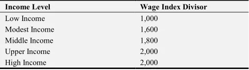
A wage index divisor3 that was based on judgment and reflects the relative wage differences across income categories was then derived (Table 3). The ratio of the wage index to assumed household income is highest for low income households and lower for high income households. Assuming that while the wage index assigned was based on judgment, it is not used to compute VoT for each category. Relative wage indices were used along with the income category frequency to match the calculated overall VoT for the El Paso metropolitan statistical area.

Table 3. Estimated Wage Index Divisor.

Income Level Wage Index Divisor

Low Income 1,000

Modest Income 1,600

Middle Income 1,800

Upper Income 2,000

High Income 2,000

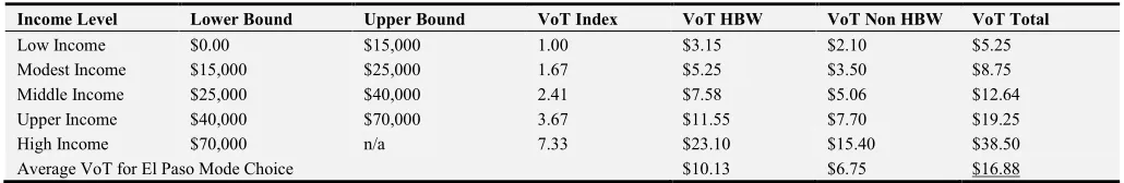
The mean household income was divided by the wage index divisor to get a wage index for each income category. The wage index was then multiplied by the frequency to derive a percentage of wage index, which in turn were summed to get a calculated VoT of $25.43. An adjustment factor was derived by dividing the mean hourly wage by the calculated VoT, which translated to a value of 0.7.4 The wage index is multiplied by the adjustment factor and the weighted percentage of trip purpose to get the VoT for each income category. The average of those VoT categories is the actual VoT for the El Paso region per trip purpose, and the summation of those two values is the final average VoT for El Paso that equates to $16.88 as shown in Table 4.

3 Wage index divisor

(7)

124 American Journal of Traffic and Transportation Engineering 2019; 4(4): 118-131

Table 4. Income Segment Assumed VoT.

Income Level Lower Bound Upper Bound VoT Index VoT HBW VoT Non HBW VoT Total

Low Income $0.00 $15,000 1.00 $3.15 $2.10 $5.25

Modest Income $15,000 $25,000 1.67 $5.25 $3.50 $8.75

Middle Income $25,000 $40,000 2.41 $7.58 $5.06 $12.64

Upper Income $40,000 $70,000 3.67 $11.55 $7.70 $19.25

High Income $70,000 n/a 7.33 $23.10 $15.40 $38.50

Average VoT for El Paso Mode Choice $10.13 $6.75 $16.88

3.5. Household Surveys—El Paso MPO

The El Paso MPO uses an official TDM that was developed for long-ranged infrastructure improvements and for conformity analysis. The TDM for the border region, termed as the Horizon Model, was developed for the El Paso County in Texas and small portions of Dona Ana and Otero Counties in New Mexico. The model base year was 2007 and included forecast years of 2010, 2020, 2030, and 2040.

The passenger car VoT for the Horizon Model was calculated from the 2009 household travel survey of the El Paso area. For each trip purpose, the average VoT was derived by aggregating individual VoTs for the survey sample and then weighted by the number of trips. The peak periods

were identified using the survey data. Based on available demographic data, 60 percent of the average hourly wage rate was used as the base VoT. The hourly wage rates in the study area were approximated to be $18.17 by using the median household income of $36,333 divided by an assumed number of 2000 total hours worked in a calendar year and the average workers per household used was 1.16. The average VoT across all trip purposes and income groups was calculated to be $9.43 (in 2007 dollars). Table 5 shows the passenger VoT for the Horizon Model in 2007 dollars. The VoT for the non-home-based external local trip purpose was assumed to be the same as the non-home-based trip purpose VoT. Forecasting those values to 2016 dollars is shown in Table 6 with an average overall VoT of $12.88.

Table 5. Horizon Model Passenger VoT (2007).

Trip Purpose Income Groups 1–3 Income Groups 4–5

Home-based-work $10.68 $13.62

Home-based non-work $8.96 $11.66

HNB Non-home- based $9.46 $12.60

Non-home-based external Local $9.46 $12.60

Average VoT = $11.13

Table 6. Horizon Model Passenger VoT (2016).

Trip Purpose Income Groups 1–3 Income Groups 4–5

Home-based-work $12.16 $15.51

Home-based non-work $10.20 $13.27

HNB Non-home- based $10.77 $14.34

Non-home-based external Local $10.77 $14.34

Average VoT = $12.88

3.6. Simulation-Based Modeling Approach (Field Data)

We developed a simulation-based DTA model derived from the official El Paso MPO TDM.5 DTA is a time-dependent methodology that captures travelers’ route choice behavior as they traverse from origin to destination. The objective function (termed dynamic user equilibrium [DUE]) is based on the idea of drivers choosing their routes through the network according to their generalized travel cost experienced during the simulation. A generalized cost includes both travel time and any monetary costs (e.g., tolls) or other relevant attributes associated with a roadway. An iterative algorithmic procedure attempts to establish DUE conditions by

5 El Paso 2040 Horizon Model was developed by the Alliance Transportation Group.

assignment of vehicles departing at the same time between the same origin-destination pair to different paths. At any given point and after much iteration, travelers learn and adapt to the transportation network conditions. The model can analyze high-occupancy vehicles, toll lanes, managed lanes, and congestion pricing and incident management. Roadways are defined in terms of functional classification, which is a system of categorizing roadways and highways by their function in the network hierarchy.

(8)

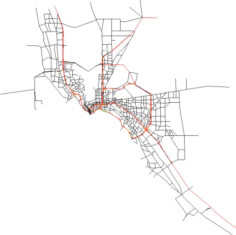
Jeffrey Shelton and Peter Martin: Determining Optimal Tolling Rates for Border Regions Using Dynamic Modeling Methods 125

Figure 4. El Paso Horizon Network.

Several data sources are used to calibrate the simulation based DTA model including speed profiles, signal timing inventories, and traffic counts. Speed profiles are used to help calibrate the traffic flow model algorithms in the DTA model, which govern how traffic flows on various roadway types. Signal timings were provided by the City of El Paso, where major arterials and diamond interchanges were coded to actual conditions. Remote areas of the city or areas with lower traffic volumes had default 2 or 3-phase signal settings. Traffic counts were used to help calibrate the demand to existing conditions. The demand matrices must be updated to reflect traffic counts throughout the region. We used a combination of RHiNo6 data provided by TxDOT and actual counts collected in the field to calibrate the final demand tables. Demand tables were calibrated without toll lanes in place to reflect before conditions. Once the matrices were calibrated to existing conditions, the toll lanes were activated to determine how many vehicles would switch their route from the general purpose lanes to the express lanes.

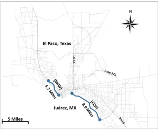
Figure 5. Cesar Chavez Express Toll Lanes [27].

Traffic counts of vehicles using the tolls lanes over a 24-hour period were obtained from the Camino Real Regional

6 Roadway Highway Inventory Network annual report published by TxDOT.

Mobility Authority (CRRMA). The Cesar Chavez toll lanes have two toll plazas in each direction where toll fees are imposed on vehicle with egress/ingress access points throughout the corridor (Figure 5).

From the data provided by the General Engineering Consultant to the CRRMA, traffic counts and toll revenue were obtained for vehicles using the express lanes for a typical workday. Traffic counts are taken at each toll plaza where vehicles are charged a distance-based toll fee. Toll rates during 2016 were $0.10/mile for the entire 8.9-mile corridor so the maximum toll fee imposed per directional trips was $0.89. Figure 6 shows the daily toll road usage in the east and westbound directions. Toll revenue generated during that day equated to $661.08 eastbound and $2,848.83 in the westbound direction.

Figure 6. Cesar Chavez—Express Lanes Daily Usage (vehs).

The DTA model was run for a 24-hour time period using the 2016 VoTs from the TxDOT road user cost approach using the CPI adjusted values ($17.52 for cars) and compared to the actual counts provided by the CRRMA general engineering consultant. An iterative process was used to vary the VoT for passenger cars (trucks are restricted from the express lanes) and compared volume results.

Given that the highest directional volume on the express lanes occurs during the morning peak period for HBW trips, the westbound numerical values were used as a basis for comparison. After multiple iterations, the VoT closest to actual field counts were converging with values lower than base line. Simulation results showed a VoT that most represents actual field counts provided by the CRRMA is $15.77, which has a volume equivalent approximately 5 percent lower than observed values in the field. The $15.77 VoT is lower than the base line VoT value used from the TxDOT road user cost adjusted using CPI approach (Table 7).

Table 7. Simulation VoT Results.

Percentage ∆ VoT WB Volumes Percent Difference

70% $12.26 1685 -15.3%

80% $14.12 1742 -12.0%

90% $15.77 1877 -4.6%

100% (Base) $17.52 1965 -

110% $19.27 2088 6.1%

120% $21.02 2411 20.4%

(9)

3.7. Existing Approaches Comparison

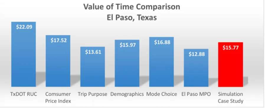
Various approaches were used to calculate a quantitative value that would be representative of the City of El Paso VoT, and then we compared those varied approaches to a simulation-based approach using the Cesar Chavez express lanes as a case study. TxDOT road user cost VoT used in A+B bidding had the highest value at $22.12, while the El Paso MPO household surveys used in the development of the regional TDM had the lowest VoT for the border region at $12.67. The weighted trip purposed approach was also lower than the value generated by the DTA model while the CPI, demographics, and CS approaches all had VoT values higher

than the DTA model.

The simulation-based approach provides the highest degree of accuracy when compared to the alternate approaches given that the DTA model uses real-world traffic volumes on the express lanes, and through an iterative process, adjusts the VoT to match simulated volumes to real data. Therefore, the modeled approach used to calculate the VoT has the highest confidence level of all approaches taken. Figure 7 outlines the various VoTs calculated and compared to the simulation-based modeling approach. Which value is correct? Further search is needed to analyze the impacts from zonal-based VoTs assessment.

Figure 7. Final Calculated VoT Comparison.

4. Static and Dynamic Pricing

Static pricing refers to a set toll rates that does not fluctuate during the day, but can charge different prices to different user classes (e.g., cars and trucks). Here, trucks are not allowed to enter tolled facilities. The toll charging system can also be defined as either link-based where vehicles are charged a fixed fee upon entering the toll lanes (e.g., toll collection booth) or distance-based where vehicles are charge a fee upon completion of their trip. This is based upon the total distance traveled. Here, we use distance-based tolling.

In order to analyze dynamic pricing, we use a congestive-responsive pricing algorithm that analyzes congestion levels in incremental time periods. The dynamic pricing algorithm has a minimum speed threshold on the toll lanes to dictate toll rate increases. If congestion levels increase on the toll road to a point where the defined minimum speed is compromised, the model increases the toll rate to deter some vehicles from entering. The DTA model analyzes speeds in 5-minute intervals and adjusts toll levels accordingly. Toll rates are analyzed for a 24-hour period to ultimately help derive a time-dependent toll rate schedule.

The goal of the dynamic pricing algorithm is to maximize revenue of vehicles while maintaining the predefined targeted minimum target speed. During periods of light congestion, minimum toll rates apply to all vehicles entering the toll

facility. If congestion builds to the point where the speed on the toll lanes drops below 45 mph, the toll rate incrementally increases until vehicles can reach the minimum speed. The VoT plays a critical role in the generalized cost calculation when assigning the time-dependent shortest paths at each time-step.

4.1. Economic Relationship

Toll revenue analysis suggests that incremental increases in toll rates will start to deter vehicles from entering the facility. Sometimes a situation can arise where the number of vehicles using the toll road will decrease as toll rates increase, yet the amount of revenue will continue to increase. The literature review suggests that demand has an elasticity of approximately 35 percent. For example, if 10,000 vehicles are on a one-mile toll facility at a certain time with a toll rate of $0.20/mile, the total revenue generated would be $2,000. So a 100 percent increase in toll rate (from $0.20 to $0.40/mile) would reduce the total number of vehicles to 6,500. The resulting revenue generated would still increase to $2,600. However, toll rates will undoubtedly reach a point where they are too expensive, and revenue will plateau before declining [28].

4.2. Optimal Toll Rates

(10)

into account the economically deprived region when compared to other Texas cities. Optimal toll rates are defined as the maximum toll rate to charge (that maximizes profits) for a defined VoT that is reflective of the socio-demographics of the border region—El Paso, Texas. We assumed that home-work and work-home related trips carry the most value to commuters—even for the lower median income residents in El Paso. Therefore we use the full VoT for home-work and

work-home trips and discounted all other trips by 50 percent. Figure 8 outlines both full and discounted VoT and how incremental increases in toll revenue will plateau before declining. The toll rate at the plateau is the maximum toll rate. This is the maximum toll rate (ξ , the value that TxDOT would like to achieve to pay back bonds. The optimal toll rate (ξR) falls below the maximum value.

Figure 8. Revenue vs. Toll Rate.

5. Tolled Scenarios

Toll road sections were derived from the El Paso MPO TDM and segregated into distinct sections. Border Highway West (BHW) extends from the downtown Santa Fe Bridge to just south of the Sunland Park collector/distributor roadway. Cesar Chavez Highway (CCH) parallels the Rio Grande River

and extends from the Zaragoza port of entry to just east of the Bridge of the Americas. The IH 10 toll road is programmed to open after 2020. No other future toll roads are modeled. For both the static and dynamic toll rate analyses, we used the weight trip purpose approach for the value of time ($13.61) for passenger cars. Figure 9 outlines all modeled toll road sections

(11)

5.1. Static Toll Rate Comparison—Results

Optimal toll rates for each defined road section are modeled using an iterative process of varying toll rates with a static toll rate algorithm. Minimum toll rates for off-peak hours are set at $0.08/mile and modeled for a 24-hour period. Toll rates are then incrementally increased from $0.08 to $0.50 per mile using the modified VoT derived from the weighted average by trip purpose approach.

Figure 8 shows revenue versus toll rates graphed where the optimal toll rate for each section is highlighted. As the toll rate is increased, revenue increases to a point where will plateau before declining. This inflection point is considered the “optimal” toll rate for the defined VoT of the border region. BHW in the westbound (WB) direction shows an increase revenue until it reaches $0.14/mile. This section had the highest toll rate/mile when compared to other sections with daily revenue over $10,000. BHW in the eastbound (EB) direction never has an incline in revenue. This means that the

optimal toll rate could be below the minimum threshold of $0.08/mile. Conversely, minimum toll rates apply to all sections so the optimal toll rate should be the minimum. One would assume that optimal tolls rates would be similar for the EB and WB directions of same roadway given directional traffic (i.e. inbound during the morning peak versus outbound during the afternoon peak). However, the morning peak period (WB) is concentrated during two to three hours of traffic where vehicles are willing to pay more to reduce their travel time.

CCH in the EB direction shows an optimal toll rate of $0.10/mile, while the WB direction indicates an optimal toll rate of $0.12/mile. These optimal toll rates are more similar than BHW so traffic is distributed more evenly during the morning and afternoon peak periods. This approach took into consideration the variability of traffic congestion during a 24-hour period. Toll rates were not able to fluctuate throughout the day.

Figure 10. Optimal Toll Rates—Static.

5.2. Dynamic Toll Comparison—Results

To obtain a dynamic optimal toll rate, we define minimum

and maximum thresholds while running the

congestive-responsive tolling algorithm. Toll rates are incrementally adjusted every 15 minutes by the algorithm, based on the operating speed of the toll lanes. If the speed drops below the minimum threshold of 45 mph, toll rates are

increased to discourage additional volume from entering the facility and promote travel time reliability. The minimum toll rate is $0.08 as defined by the Camino Real Regional Mobility Authority (CRRMA). The CRRMA was created to assist in establishing a comprehensive transportation system with the El Paso border.

(12)

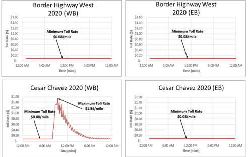
lanes never dropped below the minimum threshold of 45 mph. This is indicative of the amount of congestion needed to warrant a rate increase (i.e., the minimal toll rate set too high). Vehicles are using alternative routes without a monetary charge to reach their respective destinations. CCH in the WB direction, however, did show an almost instantaneous increase

to $1.56/mi during the morning peak period and gradually decreased as congestion levels diminished after the morning rush hour, as shown in Figure 11. 7:00 to 8:00 AM is the highest peak hour travel period. Subsequent WB morning peak hour traffic diminishes. This pattern is consistent with the directional flow of traffic during the AM period in El Paso.

Figure 11. Optimal Toll Rates—Dynamic.

6. Discussion

We used two different approaches to derive optimal toll rates for a border region—both use a generalized cost function for assignment of vehicles. The generalized cost function includes travel time and the toll rate. The static tolling approach uses incremental increases in toll rate (during each simulation run) until maximum revenue is achieved and any subsequent increases will decrease revenue. This plateaued maximum point is considered the optimal toll rate.

The dynamic congestive-responsive approach uses a minimum threshold travel speed to dictate toll rates. Congestive-responsive tolling showed that the minimum toll rate of $0.08/mile we set was too high for all corridors except CCH in the WB direction. The CCH WB direction toll rate exceeded $1.50/mile during the morning peak period and gradually decreased as traffic levels gradually declined.

Given that the static toll rates do not fluctuate during the assignment process, congestion levels at the time vehicles reach the toll lanes is the only governing factor. However, the dynamic tolling algorithm is continually updating toll rates

based on the congestion levels and the speeds vehicles are traveling inside the toll lanes. This implies that vehicles traveling through toll lanes are continually assigned to and from alternate routes (non-tolled routes) to keep the integrity of the toll lanes operating efficiently. More importantly, this means that the non-tolled lanes will continuously increase in congestion compared to the static approach. While the VoT is constant between both approaches, this variable has the greatest influence to revenue generated.

(13)

congestion levels in and around toll lanes.

Many low income individual’s VoT may be higher, because of child-care penalties or tardiness to work, which may result in job loss. In these cases, the consequences of being late will exceed the cost of the toll modeled. There is no consensus on suitable performance indicators to measure the equity impacts of toll roads.

The two modeled approaches showed differences in optimal toll rates. Which approach is more representative of the socio-demographics of a border region? The CRRMA recently changed the CCH toll road to a non-tolled facility. This was due to lack of toll revenue generated. The revenue generated was only enough to cover the operating and maintenance fees—not bond obligations [29]. It is apparent that border regions with a lower VoT are particularly sensitive to toll rates.

There are still gaps that need to be addressed that will provide more robust conclusions as they relate to optimal toll rates. An additional underlying question is whether one’s perceived VoT will change mid-trip given changing circumstances (e.g. emergency call while in the middle of a trip) and how that will influence use of toll roads. In addition, transportation planning decisions can have significant and diverse equity impacts. In particular, congestion and road pricing have raised equity concerns. Notably, the toll imposed on managed lanes on US highways affects drivers’ income. This is especially true for low-earning individuals who devote a large portion of their available budget on transportation. Therefore, any policy or project assessment should take into consideration the so-called “income effect.” [30].

7. Conclusion

The two tolling algorithms showed differences in optimal toll rate calculations. The static toll approach does not change the toll rate throughout the simulation time horizon (24-hours) so this only shows a constant value that drivers are willing to pay. The dynamic tolling algorithm has the flexibility to fluctuate during the 24-hour time horizon. This is apparent on the CCH WB direction where congestion levels rise dramatically during the morning rush hour. Which one of these approaches is correct? The dynamic tolling algorithm calculates the instantaneous toll rate based on congestion levels every 15 minutes. When the CCH WB (dynamic tolling approach) was averaged for the entire 24-hour period, the toll rate equates to $0.26/mile. This is still more than double when compared to the static algorithm.

The question posed by this research is whether the static or dynamic tolling algorithm reflects a more realistic representation of driver’s willingness to pay. The dynamic tolling algorithm prediction is more representative of the optimal tolling rate for the border region—with the exception of CCH WB. It was able to show that $0.08/mile was too high for 3 out of the 4 tolled sections in El Paso.

The concept of the trip purpose as it relates individuals VoT must be considered. Future research should address how zone-based and/or trip purpose can influence usage of toll roads. In addition, unforeseen circumstances (e.g., traffic

accidents or impending emergencies) that occur in the middle of a trip may influence the route one has chosen. This brings to question whether one’s VoT will change halfway through their trip and whether diversion to a tolled facility would occur. If this is the case, how can that be captured with existing planning models that currently forecast toll revenue? More importantly, should MPO’s employ a more comprehensive approach for calculating the VoT for the region?

References

[1] Klein, D., “The Voluntary Provision of Public Goods? The Turnpike Companies of Early America,” Economic Inquiry 28, pp 788 -794, October 1990.

[2] Wardman, M., G. Whelan, B. Vaughan, P. Murphy, G. Hyman, Modeling the Demand for Toll Roads in the UK, Proceedings of the European Transport Conference, Leiden, The Netherlands, Oct 17-19, 2007.

[3] Parkany, E., “Environmental Justice Issues Related to Transponder Ownership and Road Pricing,” Journal of the Transportation Research Record, Vol 1932, pp 97-108, Washington DC, 2005.

[4] Bain, R., Credit Risk Analysis-Toll Road Traffic & Revenue Forecasts: An Interpreter’s Guide, First Edition, Publicaciones Digitales SA, Seville, 2009. ISSB: 978-0-9561527-1-8. [5] Florida Department of Transportation, Revenue Forecasting

Guidebook, July 2018.

https://fdotwww.blob.core.windows.net/sitefinity/docs/default -source/content/planning/revenueforecast/revenue-forecasting-guidebook.pdf?sfvrsn=b40e9ddc_0.

[6] Li, Zheng, and David A. Hensher, “Toll Roads in Australia: An Overview of Characteristics and Accuracy of Demand Forecasts,” Transport Reviews 30 541-569, 2010.

[7] Li, Zheng, and David A. Hensher, “Estimating Values of Travel Time Savings for Toll Roads: Avoiding a Common Error,” Journal of Transport Policy, Vol 24 1-10, 2012.

[8] Flyvbjerg, B., M. K. S. Holm, and S. Buhl, “Inaccuracy in Traffic Forecasts,” Transport Reviews 26 (1) 1-24, 2006. [9] National Cooperative Highway Research Program, “Estimating

Toll Road Demand and Revenue: A Synthesis of Highway Practice: Synthesis 364,” Transportation Research Board, Washington DC, pp 19-35, 2006.

[10] Vassallo, J. M., A. Sánchez, “Subordinated Public Participation Loans for Financing Toll Highway Concessions in Spain,” Transportation Research Record 1996, Transportation Research Board, Washington, D. C., pp 1-8, 2007.

[11] Alasad, R., Dynamic Modelling of Demand Risk in PPP Infrastructure Projects: The Case of Toll Roads, Dissertation: Heriot-Watt University, School of Energy, Geoscience, Infrastructure & Society; August 2015.

(14)

[13] Hensher, D., and P. Goodwin, “Using Values of Travel Time Savings for Toll Roads: Avoiding Some Common Errors,” Journal of Transport Policy, Vol 11 171-181, 2004.

[14] Joksimovic, D., Bliemler, M. and Bovy, P. Optimal toll design problem in dynamic traffic networks with joint route and departure time choice. Proceedings of the 84th Annual Meeting of the Transportation Research Board, Washington, DC. 2005. [15] Chiu, Y-C, J. Bottom, M. Mahut, A. Paz, R. Balakrishna, T.

Waller, and J. Hicks, A Primer for Dynamic Traffic Assignment. Transportation Research Board, 2010.

[16] Sloboden, J., V. Alexiadis, Y-C. Chiu, and E. Nava, Traffic Analysis Toolbox Volume XIV: Guidebook on the Utilization of Dynamic Traffic Assignment. Washington, D. C.: Federal Highway Administration, 2012.

[17] Ben-Akiva, M., M. Bierlaire, H. Koutsopoulos, and R. Mishalani, DynaMIT: A Simulation-Based System for Traffic Prediction, DACCORD Short Term Forecasting Workshop, Delft, The Netherlands, Massachusetts Institute of Technology, Intelligent Transportation Systems Program, February 1998. [18] Zhang, Y., B. Atasoy, M. Ben-Akiva, Calibration and

Optimization for Adaptive Toll Pricing, Transportation Research Board 97th Annual Meeting, 2018, Annual Compendium of Papers, Washington DC. URL: https://trid.trb.org/view/1496996.

[19] Wang, S., B. Atasoy, M. Ben-Akiva, Real-Time Toll Optimization Based on Predicted Traffic Conditions, Thesis: Masters of Science in Transportation, Massachusetts Institute of Technology, Department of Civil and Environmental

Engineering, 2016. URL:

https://dspace.mit.edu/handle/1721.1/104321.

[20] Li, W., D. Cheng, R. Bian, S. Ishak and O. A. Osman, "Accounting for travel time reliability, trip purpose and departure time choice in an agent-based dynamic toll pricing approach, " in IET Intelligent Transport Systems, vol. 12, no. 1, pp. 58-65, 2 2018. DOI: 10. 1049/iet-its.2017.0004. URL: http://ieeexplore.ieee.org/stamp/stamp.jsp?tp=&arnumber=82 67183&isnumber=8267173.

[21] Hensher, D., and J. Rose, Tollroads are only part of the overall trip: The error of our ways in past willingness to pay studies, Springer Science+Business Media 819-837, 2013.

[22] Hensher, D., C. Ho, and W. Liu, “How Much is Too Much for Tolled Users: Toll Saturation and the Implications for Car Commuting Value of Travel Time Savings,” Transportation Research Part A: Transportation Research Board 601-624, 2016.

[23] Daniels, G., W. Stockton, R. Hundley, “Estimating Road User Costs Associated with Highway Construction Projects: Simplified Method,” Transportation Research Record, Journal of the Transportation Research Board, 2000. 1732: P 70—79. [24] Wardman, M., “A Review of British Evidence on Time and

Service Quality Valuations,” Transportation Research Part E: Logistics and Transportation Review, Vol 37, Issues 2-3, pp 107-128, April-July 2001. ISSN 1366-5545, DOI: 10.1016/S1366-5545 (00) 00012-0.

[25] Santos, A., N. McGuckin, H. Nakamoto, D. Gray, S. Liss, Summary of Travel Trends: 2009 National Household Travel Survey, US Department of Transportation, Federal Highway Administration, Report No. FHWA-PL-11-022, 2009. [26] National Household Travel Survey: Our Nation’s Travel.

Oakridge National Labs, 2009.

https://nhts.ornl.gov/tools/pt.shtml.

[27] Camino Real Regional Mobility Authority, 2019. https://www.crrma.org/.

[28] Beaty, C., M. Burris, and T. Geiselbrecht, Toll Roads, Toll Rates and Driver Behavior, FHWA/TX-13/0-6737-1, Editor 2012, Texas A&M Transportation Institute: College Station. [29] Texas Transportation Commission, Meeting Minutes of Public

Hearing, Item 8: Toll Roads, Section (a): El Paso County. Austin, Texas, July 17, 2017. URL: https://ftp.dot.tx.us/pub/txdot/commission/2017/0727/minutets .pdf.

[30] Cirillo, C., J. B. Vicente, Evaluating Equity Issues for Managed Lanes” Methods for Analysis and Empirical Results, Final Report, March 2019, US Department of Transportation, Federal Highway Administration, Report No.

69A43551747123. URL: