An Efficient Approximation Method for Calculating
Confidence Level of Negative Survey
Ran Liu, Jinghui Peng, Shanyu Tang∗
School of Computer Science, China University of Geosciences, Wuhan, China
Abstract
The confidence level of negative survey is one of the key scientific problem-s. Present work uses generation function to analyse the confidence level, and uses a greedy algorithm to calculate that, which is used to evaluate the dependable level of negative survey. However, the present method is low efficiency and complex. This study focuses on an efficient approximation method for calculating the confidence level of negative survey. This approxi-mation method based on central limit theorem and Bayesian method can get the results efficiently.
Keywords: Privacy protection, Data collection, Negative survey,
Confidence Level, Bayesian method
1. Introduction
Artificial Immune System simulates the mechanism of biology immune system to model and design effective algorithm for solving some complex issues. Negative selection principle [1] is one of the unique mechanisms of biology immune system, and the implication of negative selection principle
is that the immaturity T cell dies if it matches with itself as it grows, and it
survives if it mismatches with itself. Inspired by negative selection principle,
the negative selection algorithm [2] is proposed and can be used for network security, virus detection [3, 4] and anomaly detection [5].
∗Corresponding author: Tel: 86-27-67848563.
Email addresses: [email protected](Ran Liu), [email protected]
Similarly, the negative survey [6], which is inspired by negative selection principle, is a novel and promising indirect question method for information security and enhancing privacy in collecting sensitive data and individual
privacy [7]. Negative surveys consist of a question andc(c≥3) categories for
the interviewees to select. In contrast to traditional surveys, the participants
are required to select a category that does not agree with the fact [6, 8],
i.e. randomly select a category from the other c−1 unreal categories. For
convenience, it defines positive category as the category that agrees with the
fact, whilenegative category as the otherc−1 categories that does not agree
with the fact [6].
The negative survey method can attain privacy protection with lower power and higher degree, and boost participants’ confidence. The main cal-culation of collecting sensitive data with negative survey is reconstructing the corresponding positive survey in the central processor. The privacy preserv-ing properties of negative survey do not rely on anonymity, cryptography or any legal contracts, but rather participants not revealing their own privacy information. And the negative survey method is applicable to collecting data at a high speed in low-powered mobile devices such as smart phones, tablets and so on [9].
The positive survey can be reconstructed from a result of negative survey.
For a survey consist of a question and c(c≥3) categories forn interviewees
to select, a negative survey result isR = (r1, r2, ..., rc), whereri is the results
of category i in negative survey. Meanwhile, the original positive survey
is T = (t1, t2, ..., tc), where ti is the number of interviewees belonging to
category i. Define vi,j as the probability that category i is chosen given
that a respondent positively belongs to category j, where Pc
i=1vi,j = 1 and
vi,i = 0. Define the probability matrix as V as Formula (1), and R = T V
and T =RV−1. In consequence, the positive survey T can be reconstructed
from a negative survey R.
V =
0 v1,2 · · · v1,c
v2,1 0 · · · v2,c
... ... ... ...
vc,1 vc,2 · · · 0
(1)
Generally, vi,j|i6=j = 1/(c−1), which means the probability of selecting
probabilities of selecting negative categories (i.e. vi,j) follow a Gaussian
dis-tribution centered at the corresponding positive category. The GNS could attain higher accuracy but lower ability of privacy protection.
The traditional reconstructing method in [6] may lead the reconstructed positive survey with negative values. Based on the problem, two method [11] were proposed for reconstructing positive survey which had no negative values. In [12], Bao et al. proposed a greedy algorithm for calculating the confidence level, which is analysed in generating function. But this method is low efficient and complex, and couldn’t achieve the high efficiency of negative survey.
In this study, an efficient approximation method is proposed to calculate the confidence level of negative survey. This work reinforce the efficiency of negative survey.
In the remainder of this study, Section 2 introduces the related work of this study. Section 3 describes the problem in this study. Section 4 describes the efficient approximation method. Section 6 discusses some existing prob-lems of this approximation method and Section 7 concludes the whole study.
2. Related Work
In this study, the probability of selecting negative categories follows
u-niform distribution (i.e. vi,j|i6=j = 1/(c− 1)) as general negative survey
in [6, 8, 11, 12]. So in this section, the related work of negative survey [6, 8, 11, 12] is introduced. For convenience, some definitions are given in Figure 1.
Define nas the number of interviewees participating the negative survey,
and c as the number of categories. The results of the negative survey are
R = (r1, r2,· · · , rc), where ri(1≤ i ≤ c, c ≥ 3) represents the total number
of participants who select thei-th category in the negative survey. Similarly,
the real positive survey is T = (t1, t2,· · · , tc), andn=Pci=1ri =Pci=1ti. In
[6, 8], the reconstructed positive survey can be calculated by Formula (2). In
this study, a positive category i, which has n interviewees, c category, and
the proportion of category i is pi, is written as P S(n, c, pi) for simplicity.
And the corresponding negative category is written as NS(n, c, qi).
(
ˆ
tj =n−(c−1)rj
ˆ
pj = 1−(c−1)qj
n: the number of interviewees for surveys
c: the number of categories in surveys
ri : the number of interviewees selecting category i in negative survey
qi : the proportion of negative categoryi(1≤i≤c), i.e. qi =ri/n
ti : the original number of interviewees in positive category i
ˆ
ti : the estimated number of ti
R: the participant vector, i.e. R= (r1, r2,· · · , rc)
T : the participant vector, i.e. T = (t1, t2,· · · , tc)
pi : the proportion of positive category i(1≤i≤c), i.e. pi =ti/n
ˆ
pi : the estimated number of pi, i.e. ˆpi = ˆti/n
Figure 1: The definitions in this study
Although ˆpj =E(pj), it can be observed that ˆpi <0 when qi >1/(c−1)
. Therefore, this traditional method is not practical sometimes.Following the traditional method in [6, 8], two methods were proposed for reconstructing positive survey in [11]. Method I [11] uses an iteration method to recon-struct the positive survey. The advantage of Method I is that no negative
values is in the reconstructed positive survey, i.e. ˆpi > 0(1 ≤ i ≤ c). But
this method only use an implicit function to reconstruct the positive survey approximatively. And the accuracy of this method lacks of theoretical basis. Method II [11] eliminates the negative values through adjusting the results of reconstructed positive survey. This method sets the negative value of the category in the reconstructed positive survey to 0, and then keeps the sum of the reconstructed positive survey unchanged by the proportion of the values in the other categories. This method is more efficiency than Method I, but there is no theoretical analysis of this method. In [12], the confidence level of negative survey is analysed in generation functions, and calculated in a greedy algorithm.
3. Problem Formulation
necessary and inefficient to use a generation function method to exactly cal-culate the confidence level [12] with the non-exact values reconstructed from negative survey. More importantly, it is so complicated to exactly calculate the confidence level that a greedy algorithm used [12].
This study proposes an efficient method, which is analysed by central limit theorem and Bayes method, to calculate the confidence level approximately, and this approximation method can reinforce the efficiency of negative survey. The core concept of this approximation method is using Normal Distribution to approximate the original distribution for fast calculation (more details in Section 4). The Bayes method is then used to calculate the confidence level of each category in negative survey, which is studied based on the analysis of the distribution of possible positive survey results.
4. The Efficient Method of Approximation
This section gives the proposed efficient approximation method for cal-culating the confidence level. In subsection 4.1, central limit theorem is used
to calculate the approximated distribution of qi. In subsection 4.2, the Bayes
method is used to estimate the probability density function of pi. In
subsec-tion 4.3, the confidence level is calculated based on Bayes method.
4.1. The distribution of negative survey
Theorem 4.1 gives the distribution of categoryi in negative survey when
that of positive survey is known.
Theorem 4.1. For a given positive category P S(n, c, pi)and the
correspond-ing negative category NS(n, c, qi), So qi approximately follows Normal
Dis-tribution when n goes to infinity.
lim
n→∞P
qi−µ
σ2 ≤x
=
Z x
∞
1
2πe
−t22dt (3)
where µ= 1−pi
c−1, and σ
2 = (c−2)(1−pi)
n(c−1)2 .
Proof. Consider the negative category i and calculate the probability
distri-bution ofri. In the negative survey, n(1−pi) interviewees are likely to select
the i-th category. Define the random variable Xj(j = 1,2,· · · , n−ti). If the
each Xj is independent and identically distributed, and follows the Binomial
Distribution B(n(1−pi),1/(c−1)). Let X =Pjn=1(1−pi)Xj. So ri =X, and
E(ri) =
n(1−pi)
c−1 , D(ri) =
n(c−2)(1−pi)
(c−1)2 . (4)
Owing to the De Moivre − Laplace central limit theorem, ri follows Normal
Distribution as n goes to infinity, i.e.
ri ∼N
n(1−pi)
c−1 ,
n(c−2)(1−pi)
(c−1)2
(5)
So
qi ∼N(µ, σ2) =N
1−pi
c−1,
(c−2)(1−pi)
n(c−1)2
(6)
In consequence, qi follows the Normal Distribution when n goes to infinity
and Theorem 4.1 and Formula 3 are both valid.
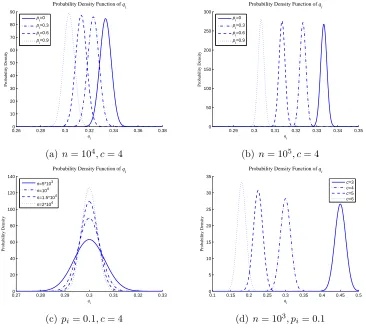
Define P(qi|pi) to be the conditional probability density function for qi
with given pi, so
P(qi|pi) =
(c−1)√nexp−n[qi(c−1)−(1−pi)]2
2(c−2)(1−pi)
p
2π(c−2)(1−pi)
(7)
Figure 2 illustrates the function cure of Formula (7) varying with pi, c, or n.
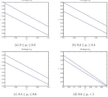
According to the character of Normal Distribution, P(|qi−µ| < 3σ) ≈
0.9974. So we can regard that maxqi =µ+ 3σ and minqi =µ−3σ. Figure 3
illustrates the range of qi for different values of pi when n = 104 and c= 4.
4.2. The distribution of reconstructed positive survey
There are some differences between reconstructing positive survey from a given negative survey and traditional method for parameter estimating. The reason is that the given result of negative survey is only one sample for its original positive survey. In consequence, we use Bayes method to reconstruct
the positive survey. The distribution of the reconstructed pi is given in the
0.260 0.28 0.3 0.32 0.34 0.36 0.38 10 20 30 40 50 60 70 80 90 qi Probability Density
Probability Density Function of q
i
p i=0 pi=0.3
pi=0.6
p
i=0.9
(a)n= 104
, c= 4
0.29 0.3 0.31 0.32 0.33 0.34 0.35
0 50 100 150 200 250 300 qi Probability Density
Probability Density Function of q
i
p i=0 pi=0.3
pi=0.6
p
i=0.9
(b) n= 105
, c= 4
0.270 0.28 0.29 0.3 0.31 0.32 0.33
20 40 60 80 100 120 140 qi Probability Density
Probability Density Function of q
i
n=5*103 n=104 n=1.5*104
n=2*104
(c)pi= 0.1, c= 4
0.1 0.15 0.2 0.25 0.3 0.35 0.4 0.45 0.5
0 5 10 15 20 25 30 35 qi Probability Density
Probability Density Function of q
i
c=3 c=4 c=5 c=6
(d)n= 103
, pi= 0.1
Figure 2: The Function Curve ofP(qi|pi) with different values ofpi,c, orn
Theorem 4.2. If a negative category is NS(n, c, qi), the probability density
function of corresponding P S(n, c, pi) is
π(pi|qi) =
e−
n[(c−1)qi−(1−pi)]2
2(c−2)(1−pi) /√1−p
i
R1
0 e
−n[(c−1)qi−(1−p)]2
2(c−2)(1−p) /√1−pdp
(8)
Proof. Define π(pi) to be the prior probability density function of pi, and
P(qi|pi) is the conditional probability density function for qi. According to
Bayes Function form of probability density function, the probability density
function of pi with given qi is the following Formula (9).
π(pi|qi) =
P(qi|pi)π(pi)
R1
0 P(qi|p)π(p)dp
0 0.05 0.1 0.15 0.2 0.25 0.26 0.27 0.28 0.29 0.3 0.31 0.32 0.33 0.34 0.35 pi qi
The Range of q
i
(a) 0≤pi ≤0.2
0.2 0.25 0.3 0.35 0.4
0.18 0.19 0.2 0.21 0.22 0.23 0.24 0.25 0.26 0.27 0.28 pi qi
The Range of q
i
(b) 0.2≤pi≤0.4
0.4 0.45 0.5 0.55 0.6
0.12 0.13 0.14 0.15 0.16 0.17 0.18 0.19 0.2 0.21 0.22 pi qi
The Range of q
i
(c) 0.4≤pi≤0.6
0.6 0.65 0.7 0.75 0.8 0.85 0.9 0.95 1
0 0.02 0.04 0.06 0.08 0.1 0.12 0.14 0.16 pi qi
The Range of q
i
(d) 0.6≤pi<1
Figure 3: The Range ofqi with probability 0.9974 (n= 104
, c= 4)
Suppose that we have no knowledge of pi. Based on Bayesian
assump-tion, the prior probability density functionπ(pi) can be considered as uniform
distribution U(0,1). On this occasion, the density function π(pi) can be
cal-culated in the following Formula (10). In addition,P(qi|pi) can be calculated
in Formula (7).
(
π(pi) = 1 0< pi <1
π(pi) = 0 otherwise
(10)
So the conditional probability density function of pi with given qi is
π(pi|qi) =
P(qi|pi)
R1
0 P(qi|pi)dpi
0 0.1 0.2 0.3 0.4 0.5 0.6 0.7 0.8 0 5 10 15 20 25 30 35 40 pi π ( pi |qi )
The Probability Density Function
qi=0.133
q i=0.233 qi=0.333
qi=0.433
(a)n= 103
, c= 4
0 0.1 0.2 0.3 0.4 0.5 0.6 0.7
0 5 10 15 20 25 30 35 40 45 pi π ( pi |qi )
The Probability Density Function
qi=0.133
q i=0.233 qi=0.333
qi=0.433
(b) n= 103
, c= 5
0.3 0.35 0.4 0.45 0.5
0 5 10 15 20 25 30 35 40 45 50 55 pi π ( pi |qi )
The Probability Density Function
n=5*103 n=104
n=1.5*104 n=2*104
(c) qi= 0.2, c= 4
0 0.1 0.2 0.3 0.4 0.5 0.6 0.7
0 5 10 15 20 25 pi π ( pi |qi )
The Probability Density Function
c=3 c=4 c=5 c=6
(d) n= 103
, qi= 0.2
Figure 4: The Function Curve ofπ(pi|qi) with different values ofqi,c, or n
Combing Formula (7) and Formula (11), Formula (8) can be get and Theorem 4.2 is valid.
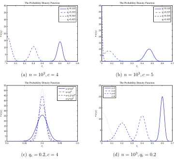
Figure 4 illustrates the function curve of π(pi|qi) for different values of
qi, n orc. Figure 4(a) and Figure 4(b) show less qi makes pi centred around
1−(c−1)qi more closely, Figure 4(c) show greaternmakes that, and Figure
4(d) shows less c makes that, too. In addition, Figure 4(a) and Figure 4(b)
also show greater qi may lead 1−(c−1)qi <0, and the corresponding pi is
0 with a great probability.
4.3. The Confidence Level
0 0.05 0.1 0.15 0.2 0.25 0.3 0.3 0.4 0.5 0.6 0.7 0.8 0.9 1 qi 1− α
The Confidence Level
δ=0.01 δ=0.02 δ=0.03 δ=0.04
(a)n= 104
, c= 4
0 0.02 0.04 0.06 0.08 0.1 0.12 0.14 0.16
0.2 0.3 0.4 0.5 0.6 0.7 0.8 0.9 1 qi 1− α
The Confidence Level
c=3 c=4 c=5 c=6
(b)n= 104
, δ= 0.01
0 0.05 0.1 0.15 0.2 0.25 0.3
0.1 0.2 0.3 0.4 0.5 0.6 0.7 0.8 0.9 1 qi 1− α
The Confidence Level
n=2*103 n=4*103 n=6*103 n=8*103
(c) c= 4, δ= 0.01
0.34 0.36 0.38 0.4 0.42 0.44 0.46 0.48 0.5 0 0.1 0.2 0.3 0.4 0.5 0.6 0.7 0.8 0.9 1 qi 1− α
The Confidence Level
n=2*103 n=4*103
n=6*103
n=8*103
(d) c= 4, δ= 0.01
Figure 5: The confidence level of estimatedpi varying withqi,c, orn
Theorem 4.3. If confidence interval length is δ, the confidence level 1−α
is
1−α=
P( ˆpi− δ2 ≤pi ≤pˆi+δ2) =
Rpˆi+δ2
ˆ
pi−δ2 π(pi|qi)dpi qi <
1−δ/2
c−1
P(0≤pi ≤δ) =
Rδ
0 π(pi|qi)dpi qi ≥
1−δ/2
c−1
(12)
where pˆi = 1−(c−1)qi, and π(pi|qi) is in Formula (8).
Proof. According to Theorem 4.2, Theorem 4.3 is valid obviously.
Figure 5 illustrates the confidence level varying with qi with different
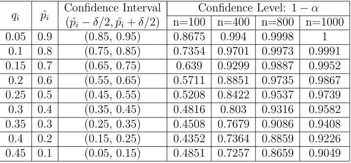
Table 1: The Confidence Level asqi< 1−δ/2
c−1 (δ= 0.1,c= 3)
qi pˆi Confidence Interval Confidence Level: 1−α
( ˆpi−δ/2,pˆi+δ/2) n=100 n=400 n=800 n=1000
0.05 0.9 (0.85, 0.95) 0.8675 0.994 0.9998 1
0.1 0.8 (0.75, 0.85) 0.7354 0.9701 0.9973 0.9991
0.15 0.7 (0.65, 0.75) 0.639 0.9299 0.9887 0.9952
0.2 0.6 (0.55, 0.65) 0.5711 0.8851 0.9735 0.9867
0.25 0.5 (0.45, 0.55) 0.5208 0.8422 0.9537 0.9739
0.3 0.4 (0.35, 0.45) 0.4816 0.803 0.9316 0.9582
0.35 0.3 (0.25, 0.35) 0.4508 0.7679 0.9086 0.9408
0.4 0.2 (0.15, 0.25) 0.4352 0.7364 0.8859 0.9226
0.45 0.1 (0.05, 0.15) 0.4851 0.7257 0.8659 0.9049
following two characters: (1) whenqi <(1−δ/2)/(c−1), the confidence level
increases withn(Figure 5(c)), and decreases withqi(Figure 5(a)) orc(Figure
5(b)). (2) when qi ≥(1−δ/2)/(c−1), the confidence level increases with qi
firstly (Figure 5(d)). Because in this case, thepi is 0 with a high probability,
the confidence level decreases severely (Figure 5(d)). These values of qi are
nearly impossible because the prior probability to attain such a large value
of qi is very low, andqi may be the survey error (if qi > µ+ 3σ as described
in subsection 4.1).
5. Simulation Experiments
In this section, some examples of negative survey (similar with that in [12]) are specially designed to verify this approximation method. In Table 1 and Table 2, the confidence level is calculated independently by category when the confidence interval (abbreviated as CI) length is 0.1. As is indicated
in Table 1, the confidence interval is ( ˆpi−δ/2,pˆi+δ/2) as qi < 1−c−δ/12 = 0.475.
In this case, the confidence level increases with n, and decreases withqi. As
shown in Table 2, the confidence level is diverse and complicated. If ˆpi <0,
then the confidence level is very small asn is large. That means an excessive
rise of qi may even be a survey error because the prior probability to attain
Table 2: The Confidence Level asqi ≥1−δ/2
c−1 (δ= 0.1,c= 3)
qi pˆi Confidence Interval Confidence Level: 1−α
(0, δ) n=100 n=400 n=800 n=1000
0.5 0 (0, 0.1) 0.7198 0.9665 0.9973 0.9992
0.55 -0.1 (0, 0.1) 0.8949 0.9995 1 1
0.6 -0.2 (0, 0.1) 0.9674 0.9933 0.2612 0.2115
0.7 -0.4 (0, 0.1) 0.9881 0.2433 0.1336 0.1171
0.8 -0.6 (0, 0.1) 0.5796 0.1568 0.1064 0.1022
Table 3: The Confidence Level asδ= 0.1 andc= 3
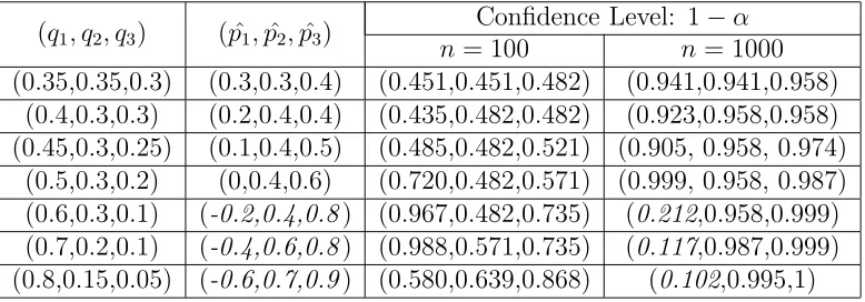
(q1, q2, q3) ( ˆp1,pˆ2,pˆ3) n= 100Confidence Level: 1n = 1000−α
(0.35,0.35,0.3) (0.3,0.3,0.4) (0.451,0.451,0.482) (0.941,0.941,0.958)
(0.4,0.3,0.3) (0.2,0.4,0.4) (0.435,0.482,0.482) (0.923,0.958,0.958)
(0.45,0.3,0.25) (0.1,0.4,0.5) (0.485,0.482,0.521) (0.905, 0.958, 0.974)
(0.5,0.3,0.2) (0,0.4,0.6) (0.720,0.482,0.571) (0.999, 0.958, 0.987)
(0.6,0.3,0.1) (-0.2,0.4,0.8) (0.967,0.482,0.735) (0.212,0.958,0.999)
(0.7,0.2,0.1) (-0.4,0.6,0.8) (0.988,0.571,0.735) (0.117,0.987,0.999)
(0.8,0.15,0.05) (-0.6,0.7,0.9) (0.580,0.639,0.868) (0.102,0.995,1)
the second method in [11] is needed to correct the reconstructed positive survey.
Table 3 shows the confidence levels of seven groups of negative survey. The confidence level includes three values, which is the confidence level of each category respectively. It is worth reminding that the confidence levels in
the last three groups of negative survey are less when n = 1000. The reason
that the probability to get such a large value of qi is rather low if n= 1000.
When n = 1000, the confidence levels of the last three groups of negative
6. Discussion
In this study, we propose an efficient approximation method for calcu-lating the confidence level of negative survey, but there are some work for future study.
Firstly, this approximation method is based on central limit theorem,
which is valid whenn is sufficiently large. However, the degree of
”sufficient-ly large” (of n) is diverse when pi has various values. So the ”sufficiently
large” cannot only be measured in n, and should be measured in both pi
and n. If npi or n(1−pi) is smaller in amount, the Poisson Distribution
is the better approximation distribution rather than Normal Distribution. In addition, Normal Distribution, which is a symmetric distribution, is used to approximate the original distribution, but the original distribution is not perfectly symmetrical.
Secondly, this method in this study analyses each category independently. The correlation of different categories should be taken into account in future
work. For example, the confidence level may be high when qi ≥ 1/(c−1).
Because the correspondingpi has a high probability to be 0. But in this case,
the sum of all the estimated pi is greater than 1, and the results is needed
for further revision.
Thirdly, the confidence interval is set to be (µ−δ/2, µ+δ/2) when qi <
1/(c−1). But strictly, π(pi|qi) is not a completely symmetrical function. So
the confidence interval may not be the smallest one.
Finally, the confidence level calculated in this study is by category inde-pendently. How to compare the two close confidence levels (such as the first two examples in Table 3) still needs to be studied further.
7. Conclusions
This study proposes an efficient approximation method for calculating the confidence level of negative survey. Normal Distribtuion is used to
ap-proximate to the distribution of qi at first, then Bayes method is used for
Acknowledgment
The project was supported by the Fundamental Research Funds for the Central Universities, China University of Geosciences (Wuhan) under Grant CUGL 140840, and the National Natural Science Foundation of China under Grant 61272469. The authors declare that there is no conflict of interests regarding the publication of this manuscript.
References
[1] S. A. Hofmeyr, S. Forrest, Architecture for an artificial immune system, Evolutionary Computation 8 (4) (2000) 443–473.
[2] S. Forrest, A. S. Perelson, L. Allen, R. Cherukuri, Self-nonself discrimi-nation in a computer, in: the IEEE Symposium on Research in Security and Privacy, 1994, pp. 202–212.
[3] J. Kim, P. J. Bentley, Towards an artificial immune system for network intrusion detection: an investigation of clonal selection with a negative selection operator, in: the 2011 Congress on Evolutionary Computa-tion(CEC’01), Vol. 2, 2001, pp. 1244–1252.
[4] G. Du, T. Huang, B. Zhao, L. Song, Dynamic self-defined immunity model base on data mining for network intrusion detection, in: the 4th International Coference on Machine Learning and Cybernetics, Vol. 6, 2005, pp. 3866–3870.
[5] Z. Ji, D. Dasgupta, V-detector: An efficient negative selection algorith-m with ”probably adequate” detector coverage, Inforalgorith-mation Sciences 179 (10) (2009) 1390–1406.
[6] F. Esponda, Negative surveys, Arxiv: math/0608176.
[7] J. Horey, M. Groat, S. Forrest, F. Esponda, Anonymous data collection in sensor networks, in: the Fourth Annual International Conference on Mobile and Ubiquitous Systems: Computing, Networking and Services, 2007, pp. 1–8.
[9] J. L. Horey, S. Forrest, M. Groat, Reconstructing spatial distributions from anonymized locations, in: 28th International Conference on Data Engineering Workshops, 2012, pp. 243 – 250.
[10] H. Xie, L. Kulik, E. Tanin, Privacy-aware collection of aggregate spatial data, Data & Knowledge Engineering 70 (6) (2011) 576 – 595.
[11] Y. Bao, W. Luo, X. Zhang, Estimating positive surveys from negative surveys, Statistics and Probability Letters 83 (2) (2013) 551 – 558.