A New Three-dimensional Assessment Model and
Optimization for Acoustic Positioning System
Lin Zhao1,Xiaobo Chen1,*, Yong Hao1, Chengcai Lv2, Lianhua Yu1
1 College of Automation, Harbin Engineering University, Harbin 150001, China; [email protected](L.Z.); [email protected](Y.H.); [email protected](L.Y.)
2 Institute of Deep-sea Science and Engineering, Chinese Academy of Sciences, Sanya 572000, China; [email protected](C.L.)
* Correspondence: [email protected]; Tel.: +86-157-6557-2980
Abstract: This paper addresses the problem of assessing and optimizing acoustic positioning
1
system for underwater target localization with range measurements only. We present a new
2
three-dimensional assessment model to assess the optimal geometric beacon formation whether
3
meet user needs. For the sake of mathematical tractability, it is assumed that the measurements of
4
the range between the target and beacons are corrupted with white Gaussian noise with variance
5
is distance-dependent. Then by adopting dilution of precision (DOP) parameters in the assessment
6
model, the relationship between DOP parameters and positioning accuracy is derived. In addition, the
7
optimal geometric beacon formation that will yield the best performance is achieved by minimizing
8
the values of geometric dilution of precision (GDOP) on condition that the position of target is known
9
and fixed. Next, in order to make sure whether the estimate positioning accuracy over interesting
10
region satisfy the precision needed by the users, geometric positioning accuracy (GPA), horizonal
11
positioning accuracy (HPA) and vertical positioning accuracy (VPA) are utilized to assess the optimal
12
geometric beacon formation. Simulation examples are designed to illustrate the exactness of the
13
conclusion. Unlike other work which only use GDOP to optimize the formation and cannot assess
14
the performance of the specified dimensions, this new three-dimensional assessment model can
15
assess the optimal geometric beacon formation in each dimension for any point in three-dimensional
16
space, which can provide users with guidance advices to optimize performance of every specified
17
dimension.
18
Keywords:acoustic positioning system; three-dimensional assessment model; positioning accuracy;
19
DOP; optimal configuration
20
1. Introduction 21
The last decade has witnessed tremendous progress in the development of marine technologies.
22
Marine robotics, for example, autonomous underwater vehicle (AUV) are becoming ubiquitous in
23
the execution of individual and military affairs. The reliable, accurate underwater positioning and
24
navigation system is quite important to the operation of AUV. The underwater positioning and
25
navigation system mainly includes inertial navigation system [1,2], geophysical navigation system
26
[3,4], visual navigation system [5,6], acoustic positioning system [7,8] and integrated navigation system
27
[9,10]. To locate targets moving in a large range and for long time, acoustic positioning system is
28
always utilized. There are lots of researchers have interest in solutions for the problem how to place
29
the beacons in two or three-dimensional space. Hong Z. [11] addressed the problem of determining
30
the optimal two-dimensional spatial placement of multiple sensors participating in a robot perception
31
task. Levanon, N. [12] studied position determination in two-dimensional scenarios by achieving
32
the lowest GDOP when range measured from beacons optimally located at the vertices of a regular
33
n-sided polygon to the target. It is noteworthy that the definition of GDOP contains the fundamental
34
relationship between measurement errors and computed position and time bias errors [13]. In this
35
paper, the definition of dilution of precision (DOP) is similar to that in [13]. Moreno-Salinas et al.
36
studied the multiple target localization with range measurements in unconstrained two-dimensional
37
scenarios [14]. Some other work also paid attention to three-dimensional scenarios. In [15], the authors
38
studied optimal sensor placement and motion coordination strategies for mobile sensor networks.
39
They investigated the determinant of the fisher information matrix (FIM) in the two-dimensional
40
and three-dimensional cases. The latter work was studied on the FIM and the maximization of its
41
determinant, in order to determine the sensor configuration that yields the most accurate positioning
42
[16]. Literature [17–20] also had close related work. More recently, in [21], Zou, Y.J. et al. assumed
43
that range measurements have different weights depending on their value and took uncertainty of
44
initial node position into consideration for the calculation of determinant of FIM. All the researches
45
above focused on the optimal beacon configuration, few focused on the assessment models and rules
46
of acoustic positioning system like assessment models and rules of global navigation satellite system
47
(GNSS). For example, in [22], the assessment models and rules of GNSS interoperability with range
48
measurements were previously presented by the author. Assessment parameters: DOP, navigation
49
satellite system precision and navigation satellite system integrity were introduced to assess the GNSS
50
performance. The work in [23] presented a study on GPS combined with Indian regional navigation
51
satellite system (IRNSS) with DOP to measure the satellite-receiver geometry related to positioning
52
accuracy. More recently, Swaszek, P. F. et al. analysed lower bounds DOP to allow users to assess how
53
well their receivers are performing respecting the best possible performance, that will be useful for
54
users to select satellites with multiple GNSS constellations, see [24] and the references therein.
55
Motivated by previous work in the area, we offer the analytic assessment model using DOP
56
parameters related to the position accuracy for the problem of assessing acoustic positioning system
57
in this paper. Then the geometric beacon placement is optimized based on target to beacons range
58
measurements only. Next, what we should take care is the values of GPA, HPA and VPA over the
59
interesting region where the sampling points taking place of the target. The document is organized as
60
follows. In Section 2, DOP parameters and positioning accuracy for the assessment model are derived,
61
the steps to assess the acoustic positioning system are listed as well. Section 3 contains the optimal
62
beacon configurations for the case where the beacons can be placed freely in both two-dimensional
63
scenario and three-dimensional scenario. The results of Section 3 are then examined in Section 4 for
64
the particular scenario, and the steps to assess the acoustic positioning system in practice are shown.
65
Finally, Section 5 contains the conclusions and further research.
66
2. Assessment model: DOP parameters and position accuracy 67
DOP parameters in literature [13] are defined as geometry factors that relate the target position
68
errors to the measurements of the ranges errors. Generally, the receiver and beacons clock both have
69
bias errors from the system time and the bias errors are a few microseconds or so, the speed of sound
70
in water is about 1500 m/s, then the measurements errors are insignificant compared to the accuracy
71
of positioning. Consequently, the DOP parameters in this paper don’t consider the clock bias errors.
72
In what follows, the position of theith beacon is(xi,yi,zi)relative to the coordinate origin, and the
73
target’s actual position coordinates(x,y,z)are considered unknown. In order to achieve the target’s
74
position in three dimensions, ideal measurements of ranges are made withn(n>3)beacons from
75
equations:
76
di= f(x,y,z) =
q
(xi−x)2+ (yi−y)2+ (zi−z)2 (1)
wherediis ideal measurement of range from theith beacon to the target without noise interference,i
77
ranges from 1 tonand references the beacons.
78
However, the measurements are always corrupted by noise. We assume that all noise sources are
79
independent and have equal variance, with this notation, the measurement model is given by:
80
Di = q
whereDiis actual measurement of range from theith beacon to the target with noise interference,ωiis
81
the measurement error taken to be a zero mean Gaussian processN(0,σ2)with covariance isσ2.
82
Assuming that the target’s position is approximately estimated as (xe,ye,ze) when the
83
measurements are corrupted by noise. However, we still use Equation (1) to estimate the position of
84
target, thus we get the expression as follows:
85
Di = f(xe,ye,ze) =
q
(xi−xe)2+ (yi−ye)2+ (zi−ze)2 (3)
We can denote the offset of the actual position (x,y,z) from the approximate position by a
86
displacement(∆x,∆y,∆z)described as:
87
x=xe+∆x
y=ye+∆y
z=ze+∆z
(4)
Substituting (4) into (1), we can get the expression:
88
f(x,y,z) = f(xe+∆x,ye+∆y,ze+∆z) (5) This latter function can be expanded about the approximate target’s position using a Taylor series:
89
f(xe+∆x,ye+∆y,ze+∆z) = f(xe,ye,ze)+ ∂f(xe,ye,ze)
∂xe ∆x+
∂f(xe,ye,ze)
∂ye ∆y+
∂f(xe,ye,ze)
∂ze ∆z+· · ·
(6)
The expansion has been truncated after the first-order partial derivatives and the partial
90
derivatives evaluate as follows:
91
∂f(xe,ye,ze)
∂xe =−
(xi−xe) Di
∂f(xe,ye,ze)
∂ye =−
(yi−ye)
Di
∂f(xe,ye,ze)
∂ze =−
(zi−ze)
Di
(7)
Substituting (7) into (6) yields:
92
di=Di−
(xi−xe) Di ∆x
− (yi−ye)
Di ∆y
−(zi−ze)
Di ∆z
(8)
For convenience, we will simplify Equation (8) by introducing new variables where:
93
axi=
(xi−xe) Di ayi=
(yi−ye) Di azi= (zi−ze)
Di
(9)
By substituting (9) into (8),ωican be determined:
94
ωi=Di−di=axi∆x+ayi∆y+azi∆z (10) Now we have three unknowns composing the vector∆u = (∆x,∆y,∆z)T and the unknown
95
quantities can be determined by solving the matrix shown as:
∆d=H∆u (11)
whereTdonates the transpose of matrix; the matrix∆dand observation matrixHare described by
97
making the definitions:
98
∆d=
ω1
ω2 .. .
ωn
(12)
H=
ax1 ay1 az1 ax2 ay2 az2
..
. ... ... axn ayn azn
(13)
If vectors(axi,ayi,azi)do not all lie in a plane, the weighting matrix(HTH)will be invertible.
99
Thus the method of least squares can be used to solve Equation (11) for∆u:
100
∆u= (HTH)−1HT∆d (14)
In fact, the ideal positioning accuracy is decided by∆u, then the covariance of∆uis obtained by
101
forming the product∆u∆uTand computing an expected value:
102
cov∆u=E∆u∆uT
=E
(HTH)−1HT∆d(HTH)−1HT∆dT
=E
h
(HTH)−1HT∆d∆dTH(HTH)−1i
= (HTH)−1HTcov(∆d)H(HTH)−1
(15)
The usual assumption is thatωiis distributed and independent, with zero mean Gaussian process whose variance isσ2. The covariance of∆dis a scalar multiple of the identity:σ2In×n, whereIn×nis then×nidentity matrix.Then the result of Equation (15) is derived as:
cov∆u=σ2(HTH)−1HTH(HTH)−1=σ2(HTH)−1 (16)
Under the stated assumptions, the covariance of the errors of the position is just a scalar multiple
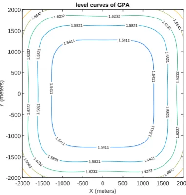
103
of the weighting matrix(HTH)−1. The covariance of ∆u is a 3×3 matrix and has an expanded 104
representation:
105
cov(∆u) =
σx2 σxσy σxσz
σxσy σy2 σyσz
σxσz σyσz σz2
(17)
The components of the weighting matrix(HTH)−1quantify how measurement errors translate 106
into components of the covariance of∆u. Express the weighting matrix(HTH)−1in component form: 107
(HTH)−1=D=
D11 D12 D13 D21 D22 D23 D31 D32 D33
(18)
unlike other work which only use GDOP to optimize the formation and cannot assess the
108
performance of any specified dimensions, more DOP parameters are presented in this paper, we
use GDOP, HDOP and VDOP to assess the optimal geometric beacon formation in each dimension for
110
any point in three-dimensional space:
111
GDOP=pD11+D22+D33=
q
σx2+σy2+σz2
σ
HDOP=pD11+D22 =
q
σx2+σy2
σ
VDOP=pD33=
p
σz2
σ
(19)
To assess the acoustic positioning system, the sampling points over interesting region are adopted
112
to take place of the approximate target’s position. Then the observation matrixHis achieved by the
113
Equation (20):
114
H=
(x1−xs)
r1
(y1−ys) r1
(z1−zs)
r1
(x2−xs)
r2
(y2−ys)
r2
(z2−zs)
r2
..
. ... ...
(xn−xs)
rn
(yn−ys) rn
(zn−zs)
rn
(20)
where(xi,yi,zi),i=1· · ·ndenote theith beacon’s position in three dimensions,(xs,ys,zs)denote the
115
sampling point’s position over interesting region in three dimensions,riis the range between theith
116
beacon and the sampling point.
117
Equation (20) is valid provided that the range measurement errors are sufficiently small so that
118
the error between sample point’s actual position and approximately estimated position can be ignored.
119
The minimum ofσisc/2f in theory, wherecis the speed of propagation of sound in the water, f is the
120
frequency of sound in the water. However,σin practice is always far larger thanc/2f. Multiplyσby
121
GDOP, HDOP and VDOP, respectively, then the GPA, HPA and VPA will be obtained, correspondingly.
122
GPA=qσx2+σy2+σz2=GDOP×σ
HPA=qσx2+σy2=HDOP×σ
VPA=σz=VDOP×σ
(21)
Compare the GPA, HPA and VPA with the user requirements and decide whether the positioning
123
accuracy meet the user requirements. If they don’t, that means more beacons are needed. If the HPA
124
don’t satisfy the user requirements, add the beacons in the horizonal plane. If the VPA don’t satisfy the
125
user requirements, add the beacons in vertical plane. If the GPA don’t satisfy the user requirements,
126
add the beacons in horizonal plane mainly.
127
According to the above analysis, the steps to assessment acoustic positioning system can be
128
summarized as follows:
129
1. Determine the optimal beacons configurations with n beacons: the beacons should be distributed
130
at the vertices of a regular n-sided polygon on the same plane. This conclusion is drawn in Section
131
3.
132
2. According to the spatial resolution needed by users, make sure the sampling points in space, then
133
compute the ranges from beacons to the all sampling points in space by Equation (1).
134
3. Define the variance of range measurements errorsσ, obtain the DOP parameters, GDOP, HDOP
135
and VDOP by the Equation (19), and compute the GPA, HPA and VPA by the Equation (21).
136
4. Define the variance of range measurements errorsσ, obtain the DOP parameters, GDOP, HDOP
137
and VDOP by the Equation (19), and compute the GPA, HPA and VPA by the Equation (21).
138
5. Determine whether increase the number of beacons into the acoustic positioning system according
139
to the compare between the ideal positioning accuracy and the users’ requirements.
3. The optimal beacons configurations with DOP parameters 141
3.1. Two-dimensional scenarios
142
This section addresses the problem of estimate beacon placement for underwater target
143
positioning in two-dimensional space, subject to the condition that the beacons and the sampling point
144
lie on the horizontal plane. In this situation,His singular so the matrixDdoesn’t exist. For the sake of
145
simplicity, and without loss of generality, the sampling point is considered to be located at the origin
146
of the inertial coordinate frame hereinafter. It is assumed that the position of theith beacon is located
147
on the point whose radius isriand the polar angle isαi, so the polar coordinates of theith beacon is
148
(ricosαi,risinαi), then the matrixHcan be simplified asH1:
149
H1=
r1cosα1
r1
r1sinα1
r1
r2cosα2
r2
r2sinα2
r2
..
. ... rncosαn
rn
rnsinαn rn
=
cosα1 sinα1 cosα2 sinα2
..
. ... cosαn sinαn
(22)
At this point, we introduce the vectors,XandY, defined as:
150
X=hcosα1 cosα2 · · · cosαn i
Y=hsinα1 sinα2 · · · sinαn
i (23)
It’s obvious that the analytical relationship of the determinant ofXandYis as follows:
151
|X|2+|Y|2=n (24)
As a consequence, defineφis the angle formed by vectorsXandY, then the weighting matrix
152
D1= (H1TH1)−1is parameterized by two vectorsXandY:
153
D1=
" ∑n
i=1cos2αi ∑in=1cosαisinαi ∑n
i=1cosαisinαi ∑ni=1sin2αi #−1
=
"
Y2 − |X| |Y|cosφ
− |X| |Y|cosφ X2
#
det(H1TH1)
(25)
The determinant ofH1TH1yields:
154
det(H1TH1) =|X|2|Y|2(1−cos2φ) (26)
Obviously, cos2φ=0 is the only feasible solution to make thedet(H
1TH1)largest that implies
155
that vectorsXandYare orthogonal. This condition makes (H1TH1)−1be a diagonal matrix and
156
det(H1TH1)can now be written as:
157
det(H1TH1) =|X|2|Y|2=|X|2(n− |X|2)≤ −(|X|2−n/2)2+n2/4 (27)
One obtains, finally:
158
HDOP≥
r n n2/4 =
r 4
n (28)
We will now make sure the beacon configurations. Define the sampling point at the center of
159
an n-sided regular polygon(n≥2), and the n beacons are placed at the vertices of a regular n-sided
160
polygon. Then coordinate of theith beacons is described as:
ricos
2π(i−1)
n ,risin
2π(i−1)
n
i=1, 2,· · ·,n (29) Then the matrixH1can be described as:
162
H1=
cos 0 sin 0 cos2π
n sin2nπ ..
. ...
cos2π(ni−1) sin2π(ni−1)
(30)
Using the Fourier summation formulas:
163
n
∑
i=1
cos22π(i−1)
n =
n 2 n
∑
i=1
sin22π(i−1)
n =
n 2 n
∑
i=1
cos2π(i−1)
n sin
2π(i−1)
n =0
n
∑
i=1
cos2π(i−1)
n =
n
∑
i=1
sin2π(i−1)
n =0
(31)
Substituting Equation (31) into Equation (25) yields:
164
D1=
"n 2 0 0 n2
#−1
=
"2 n 0 0 2n #
(32)
We now can draw the conclusion that in two-dimensional scenarios, it is clear that the beacon
165
configurations have no explicit dependence on the ranges, only related to the angles that the range
166
vectors form with the unit axes of the frame. What’s more, for position determination, based on n
167
range measurements(n> 2), the lowest possible HDOP is 2/√n. This value will occur when the
168
sampling point is on the initial point, and the n beacons are located at the vertices of regular n-sided
169
polygon. Then more optimal beacon configurations can be generated by two methods: 1) multiplying
170
the range of each beacon to the sampling point by an arbitrary positive number as long as the sampling
171
point could receive the signals from all beacons. 2) rotating the beacon formation rigidly in terms of an
172
arbitrary axis. However, the two methods can only make the lowest possible HDOP constant when the
173
sampling point is on the initial point, and the n beacons are located at the vertices of regular n-sided
174
polygon.
175
3.2. Three-dimensional scenarios
176
Similar to the two-dimensional scenarios, the sampling point is considered to be located at the
177
origin of the inertial coordinate frame hereinafter. Assume that the position of theith beacon is
178
located on the point(xi,yi,zi), and the range between the sampling point and the beacon isri =
179 q
(x2i +y2i +z2i). Define the angles(αi,βi,γi)shown as Equation (33):
180
cosαi=xi/ri cosβi=yi/ri cosγi=zi/ri
Then the coordinate of theith beacon can be defined as(ricosαi,ricosβi,ricosγi). The matrix of
181
Hbecomes:
182
H1=
r1cosα1
r1
r1cosβ1
r1
r1cosγ1
r1
r2cosα2
r2
r2cosβ2
r2
r2cosγ2
r2
..
. ... ... rncosαn
rn
rncosβn rn
rncosγn rn
=
cosα1 cosβ1 cosγ1 cosα2 cosβ2 cosγ2
..
. ... ... cosαn cosβn cosγn
(34)
It is convenient to introduce the vectorsX,YandZdefined as:
183
X=hcosα1 cosα2 · · · cosαn i
Y=hcosβ1 cosβ2 · · · cosβn i
Z=hcosγ1 cosγ2 · · · cosγn i
(35)
The relationship of the determinant ofX,YandZis shown as follows:
184
|X|2+|Y|2+|Z|2=n (36)
Computations show that Equation (18) can be rewritten as:
185
D= (HTH)−1=
|X|2 |X| |Y|cosϕ |X| |Z|cosθ
|X| |Y|cosϕ |Y|2 |Y| |Z|cosω
|X| |Z|cosθ |Y| |Z|cosω |Z|2
−1
(37)
whereϕ,θandωare the angles formed by vectorsXandY,YandZ,YandZ, respectively.
186
From Equation (37) it follows that:
187
GDOP=
s
|Y|2|Z|2(1−cos2ω) +|X|2|Z|2(1−cos2θ) +|X|2|Y|2(1−cos2ϕ)
det(HTH) (38)
The determinant of(HTH)yields:
188
det(HTH) =|X|2|Y|2|Z|2(1+2 cos
ωcosθcosϕ−cos2θ−cos2ω−cos2ϕ) (39)
We suppose a procedure inspired in the two-dimensional problem, the optimal solution is:
189
cosω=cosθ=cosϕ=0 (40)
In this situation, it follows that:
190
1−cos2ω
1+2 cosωcosθcosϕ−cos2θ−cos2ω−cos2ϕ =1
1−cos2θ
1+2 cosωcosθcosϕ−cos2θ−cos2ω−cos2ϕ =1
1−cos2ϕ
1+2 cosωcosθcosϕ−cos2θ−cos2ω−cos2ϕ =1
(41)
We now show that 1 is their minimum possible values. Without loss of generality, suppose that a
191
smaller value that clearly satisfies:
1−cos2ω
1+2 cosωcosθcosϕ−cos2θ−cos2ω−cos2ϕ <1 (42)
As it’s known to all, the determinant of symmetrical matrixHTHis not less than 0. What’s more,
193
GDOP is inexistence when the determinant ofHTH=0. Therefore, the determinant ofHTH>0 is in
194
consideration. In this situation, the above inequality is equivalent to:
195
0<2 cosωcosθcosϕ−cos2θ−cos2ϕ (43)
Because|cosω|<1, it follows that:
196
2 cosωcosθcosϕ≤cos2θ+cos2ϕ (44)
This conclusion contradicts Equation (43). Therefore:
197
1−cos2ω
1+2 cosωcosθcosϕ−cos2θ−cos2ω−cos2ϕ ≥1 (45)
Similarly, we can prove that:
198
1−cos2θ
1+2 cosωcosθcosϕ−cos2θ−cos2ω−cos2ϕ ≥1
1−cos2ϕ
1+2 cosωcosθcosϕ−cos2θ−cos2ω−cos2ϕ ≥1
(46)
In these circumstances, GDOP is computed as:
199
GDOP=
s 1
|X|2+
1
|Y|2 +
1
|Z|2 = s
1
|X|2+
1
|Y|2+
1
n− |X|2− |Y|2 (47)
Construct the binary function f(a,b)as follows:
200
f(a,b) = 1
a+ 1 b+
1
n−a−b (48)
The Hessian matrix of Equation (48) is:
201
Hessian=
"∂2f(a,b)
∂a2
∂f(a,b) ∂a∂b ∂f(a,b)
∂b∂a
∂2f(a,b)
∂b2
#
=
"2
a3 +(n−a2−b)3 (n−a2−b)3
2
(n−a−b)3 a23 +(n−a2−b)3
#
(49)
where it is easy to proof that the Hessian matrix of Equation (48) is positive definite, the minimum
202
value of f(a,b)is obtained provided that the first derivatives equal to 0:
203
∂f(a,b)
∂a =
1
(n−a−b)2− 1 a2 =0
∂f(a,b)
∂a =
1
(n−a−b)2− 1 b2 =0
(50)
From which follows that:
204
a=b= n
3 (51)
Substituting this result in Equation (36), we obtain:
|X|2=|Y|2=|Z|2= n
3 (52)
Now we determine the geometric configuration in three-dimensional scenarios. To simplify the
206
computation, we assume that the optimal beacon formations are placed on a unit sphere centered
207
at the sampling point. Inspired by the work in two-dimensional scenarios, we address the problem
208
of optimal beacon placement subject to the condition that the beacons lie on the same plane. Then
209
the beacons may be distributed at the vertices of a regular n-sided polygon, which belongs to the
210
circumference of the planez= √1
3 or on the circumference of the planez=− 1 √
3. In addition, the 211
optimal radiusR=q23. Now we give a simple proof of this geometric configuration. Firstly, rewrite
212
the positions of the beacons in polar coordinates as:
213
cosαi=xi/ri =xi cosβi =yi/ri=yi cosγi=zi/ri =zi
(53)
Because all beacons are distributed on the circumference of the plane z = √1
3 or on the 214
circumference of the planez=−√1
3. It then follows that: 215
cos2γi= 1 3
|Z|2=
n
∑
i=1
cos2γi= n 3
(54)
With the conclusion in Equation (31), we can get:
216
n
∑
i=1 xi
R 2
=
n
∑
i=1
cos22π(i−1)
n =
n 2 n
∑
i=1 yi
R 2
=
n
∑
i=1
sin22π(i−1)
n =
n 2 n
∑
i=1 xi
R yi R
=
n
∑
i=1
cos2π(i−1)
n sin
2π(i−1)
n =0
n
∑
i=1 xi
R
=
n
∑
i=1
cos2π(i−1)
n =0
n
∑
i=1 yi
R
=
n
∑
i=1
sin2π(i−1)
n =0
(55)
Therefore, we can obtain the formula as follows:
|X|2=
n
∑
i=1
(xi)2= n 2 ×R
2= n 3
|Y|2=
n
∑
i=1
(yi)2= n 2 ×R
2= n 3
|X| |Y|=
n
∑
i=1
(xiyi) =0
|Z| |X|=
r 1 3
n
∑
i=1
(xi) =0
|Z| |Y|=
r 1 3
n
∑
i=1
(yi) =0
(56)
Then Equation (37) yields:
218
D= (HTH)−1=
n
3 0 0
0 n3 0 0 0 n3 −1 = 3
n 0 0 0 3n 0 0 0 n3
(57)
Once the optimal beacon placement on a unit sphere in three-dimensional scenarios is found
219
in terms of the direction cosines achieved above, more infinite optimal beacon placements can be
220
generated by multiplying the range of each beacon to the sampling point by an arbitrary positive
221
number, as long as the sampling point can receive the signal from the beacons. The lowest possible
222
GDOP is 3/√nbased on n range measurements(n>3).
223
An interesting problem arises: whether HDOP and VDOP get the lowest value when the optimal
224
beacons configurations make GDOP lowest. The answer is no. Assume that the coordinate of theith
225
beacon is(xi,yi,z), without loss of generality, if the beacons are located on a circle centered at the
226
sampling point described as:
227
x2i +y2i =rˆ2 (58)
With the condition shown in Equations (36) and (40), HDOP and VDOP are described as:
228
HDOP=
s 1
|X|2 +
1
|Y|2 = v u u tn
− |Z|2 |X|2|Y|2 =
v u u u t
n−nrˆ2z+2z2
∑n i=1
x2
i ˆ
r2+z2 ∑ni=1 y2
i ˆ r2+z2
=
s
n(rˆ2+z2)2−nz2(rˆ2+z2) ∑n
i=1x2i ∑ n i=1y2i
=
s
n(ˆr2+z2)rˆ2 ∑n
i=1x2i ∑ n i=1y2i
(59)
VDOP=
s 1
|Z|2 = s
1 nz2z+2rˆ2
=
s 1 n
1+rˆ
2
z2
(60)
It’s shown that the vertical distancezbetween beacons and sampling point becomes larger, HDOP
229
will be larger, and VDOP will be smaller. In many practical applications of interest, however, the
230
sampling point’s depth can be measured directly with small error. Thus there’s no need to estimate it
231
with acoustic range measurements. Therefore, based on the GDOP or HDOP, we can decide whether
232
the beacons configuration meet user needs.
4. Simulation example 234
4.1. Optimal beacon placement in two-dimensional scenarios
235
If there is only one sampling point in the acoustic positioning system and known to users, section
236
3.1 shows clearly that the optimal beacons are placed at the vertices of regular n-sided polygon. Given
237
the experimental conditions, it’s necessary to estimate how good the positioning accuracy in term
238
of the beacon formation for anywhere in the acoustic positioning system. In order to achieve the
239
goal, HPA with hypothetical sampling point on a grid in a finite spatial regionAis computed. In this
240
paper, regionAwill always be rectangle. The formation is the one in which four beacons are placed at
241
p1= [2000, 2000]m,p2= [−2000, 2000]m,p3= [−2000,−2000]m,p4= [2000,−2000]m. It’s assumed 242
that all range measurements are corrupted by additive zero mean Gaussian noise with varianceσ=1
243
so that the values of HPA are equal to that of HDOP. The spatial resolution chosen is 2m×2m.
244
Figure 1.HPA in the 3D view in two-dimensional scenarios.
1.02
1.02
1.02
1.02
1.02
1.02
1.02
1.04
1.04
1.04
1.04
1.04
1.04
1.04
1.04
1.06 1.06
1.06
1.06 1.06
1.06
1.06
1.06
1.08
1.08 1.08
1.08
1.1 1.1
1.1
1.1
1.12
1.12 1.12
1.12 level curves of HPA
X (meters)
-2000 -1500 -1000 -500 0 500 1000 1500 2000
Y (meters)
-2000 -1500 -1000 -500 0 500 1000 1500 2000
The simulation results of HPA are presented in Figure 1 and 2. In Figure 1, the values of HPA in
245
3D view for regionAare shown. It’s important to note that the HPA obtained at the point of beacon are
246
computed with three other beacons, without the beacon location itself, so as to avoiddet(HTH) =0.
247
Thus, the values of HPA at these points are extra-large. In Figure 2, level curves of HPA in regionAare
248
shown. We can draw the conclusion that better performance obtained in two-dimensional scenarios is
249
within the circle of 1.02, which inspires us around the centre of the beacon is more accurate than that
250
nearby the beacon. Furthermore, the better positioning region in two-dimensional scenarios is like a
251
square, however, rotating 90 degrees to the beacon formation.
252
4.2. Optimal beacon placement in three-dimensional scenarios
253
For three-dimensional scenario, the beacons are supposed to be placed on the surface of the
254
sea, and the coordinates arep1= [2000, 2000, 0]m,p2= [−2000, 2000, 0]m,p3= [−2000,−2000, 0]m, 255
p4= [2000,−2000, 0]m. Similar to the two-dimensional scenario, all range measurements are assumed 256
to be corrupted by additive zero mean Gaussian noise with varianceσ=1. Three different levels of
257
sampling points’ height are considered for the computation of the GPA involved in the optimization
258
figuration. The depths of the sampling points are assumed to be−1000m,−2000mand−3000m,
259
respectively. The spatial resolution chosen is 2m×2m. In Figure 3 and 4, GPA values of the−2000m
260
sampling points are supplied. The other GPA values of the−1000mand−3000msampling points
261
are similar to those of−2000m. They aren’t presented in this paper due to space limitations. The
262
comparison of GPA, HPA and VPA between different sampling points’ height are provided in Table 1.
263
From Figure 3, the best theoretical accuracy is obtained at the centre of beacons. It implies the
264
target around the centre of the beacons can achieve more accurate positioning than those nearby the
265
beacons. From Figure 4, it suggests that the better positioning region in three-dimensional scenarios
266
is also like a square, similar to the beacon formation. Therefore, the beacons for acoustic positioning
267
should be located beyond the interesting region. What’s more, the better performance will be achieved
268
when the distances between beacons are larger, only if the target could receive the signals from all
269
beacons. Over the interesting region, GPA show ideal accuracies in some parts of the interesting
270
region. This fact will be of great importance to determine the number of beacons needed or whether
271
the positioning accuracy over a given area meets user needs.
272
1.5411
1.5411
1.5411 1.5411
1.5411
1.5411
1.5411
1.5821
1.5821
1.5821
1.5821 1.5821
1.5821
1.5821
1.5821 1.5821
1.6232 1.6232 1.6232
1.6232 1.6232
1.6232
1.6232
1.6232
1.6232 1.6232
1.6643
1.6643
1.6643 1.6643
level curves of GPA
X (meters)
-2000 -1500 -1000 -500 0 500 1000 1500 2000
Y (meters)
-2000 -1500 -1000 -500 0 500 1000 1500 2000
Figure 4.Level curves of HPA in three-dimensional scenarios.
For each case in three-dimensional scenarios, the minimum and maximum GPA, HPA as well as
273
VPA are computed with the optimal beacon placement. The results are shown in Table 1.
274
Table 1.Results for three different sampling points’ height.
GPAmin GPAmax HPAmin HPAmax VPAmin VPAmax
-1000m 1.5651 1.9538 1.0607 1.2862 0.9682 1.5811 -2000m 1.5000 1.7464 1.2247 1.4491 0.8602 1.0000 -3000m 1.6116 1.9274 1.4577 1.6748 0.6872 0.9539
It’s obvious shown that minimum of GPA(GDOP) is obtained when the sampling points’ height
275
is−2000m, and this value satisfied the formula 3/√n=3/√4=1.5. What’s more, the data in Table 1
276
imply that HPA(HDOP) grow proportional to the height of sampling points. However, VPA(VDOP)
277
grow inversely proportional to the height of sampling points. This conclusion is consistent with the
278
theory in section 3.2.
279
5. Conclusions 280
This paper offered a new characterization of the solutions to assess and optimize acoustic
281
positioning system. By assuming that the range measurements between the sampling points and the
282
acoustic beacons were corrupted by white Gaussian noise, the assessment parameter DOP related
283
to the positioning accuracy were derived. Then the best positioning accuracy to be obtained was
284
converted into that of minimizing the GDOP conveniently. Furthermore, unlike other work only use
285
GDOP to optimize the formation and cannot assess the performance of any specified dimensions
286
whether users satisfy, we use GPA, HPA and VPA to assess the optimal geometric beacon formation in
287
each dimension for any point in three-dimensional space. This new assessment model can provide
288
users with guidance advices to optimize performance of each specified dimension. Finally, numerical
289
simulations support the view that the methodology proposed to estimate performance of acoustic
290
system is feasible. Future work will aim at: 1) extending the methodology developed to deal with
291
time bias errors; 2) studying the performance of the acoustic positioning system on condition that the
292
beacons is in motion with ocean currents.
Acknowledgments:This work is supported by National Natural Science Foundation of China (No. 61633008, 294
No. 61374007, No. 61601262, No.61701487), Natural Science Foundation of Heilongjiang Province of China (No. 295
F2017005) and Natural Science Foundation of Hainan Province of China (No. 117212, No.417211). 296
Author Contributions:X.C. wrote the paper; L.Z. and X.C. conceived and designed the experiments; Y.H. and C.L. 297
performed the simulations; C.L. and L.Y. analyzed the data. All authors read and approved the final manuscripts. 298
Conflicts of Interest:The authors declare no conflict of interest. 299
References 300
1. Xu, J. N.; He, H. Y.; Qin, F. J.; Chang, L. B. A novel autonomous initial alignment method for strapdown 301
inertial navigation system. IEEE Transactions On Instrumentation And Measurement2017, 66, 2274-2282, 302
10.1109/TIM.2017.2692311. 303
2. Chang, L. B.; Li, Y.; Xue, B. Y. Initial alignment for a doppler velocity log-aided strapdown inertial 304
navigation system with limited information. IEEE-ASME Transactions On Mechatronics2017,22, 329-338, 305
10.1109/TMECH.2016.2616412. 306
3. Rice, H.; Kelmenson, S.; Mendelsohn, L. Geophysical Navigation Technologies And Applications. In 307
Proceedings of the Position Location and Navigation Symposium, Monterey, CA, USA, April 2006; pp. 308
618-624. 309
4. Teixeira, F. C. Novel Approaches To Geophysical Navigation Of Autonomous Underwater Vehicles. In 310
Proceedings of the International Conference on Computer Aided Systems Theory, Las Palmas de Gran 311
Canaria, Spain, February 2013; pp. 349-356. 312
5. Bonin-Font, F.; Ortiz, A.; Oliver, G. Visual navigation for mobile robots: A survey.IEEE-ASME Transactions 313
On Mechatronics2008,53, 263-296, 10.1007/s10846-008-9235-4. 314
6. Eustice, R.; Pizarro, O.; Singh, H. Visually augmented navigation for autonomous underwater vehicles.IEEE 315
Journal of Oceanic Engineering2008,33, 103-122, 10.1109/JOE.2008.923547. 316
7. Cheng, X. Z.; Shu, H. N.; Liang, Q. L. Silent positioning in underwater acoustic sensor networks. IEEE 317
Transactions On Vehicular Technology2008,57, 1756-1766, 10.1109/TVT.2007.912142. 318
8. Bayat, M.; Crasta, N.; Aguiar, A. P.; Pascoal, A. M. Range-Based Underwater Vehicle Localization in the 319
Presence of Unknown Ocean Currents: Theory and Experiments. IEEE Transactions On Control Systems 320
Technology2016,24, 122-139, 10.1109/TCST.2015.2420636. 321
9. Zhang, T.; Chen, L. P.; Li, Y. AUV Underwater Positioning Algorithm Based on Interactive Assistance of 322
SINS and LBL.Sensors2016,16, 1-22, 10.3390/s16010042. 323
10. Shabani, M.; Gholami, A.; Davari, N. Asynchronous direct Kalman filtering approach for underwater 324
integrated navigation system.Nonlinear Dynamics2014,80, 71-85, 10.1007/s11071-014-1852-9. 325
11. Hong, Z. Two-Dimensional Optimal Sensor Placement.IEEE Transactions on Systems, Man, and Cybernetics 326
1995,25, 781-792, 10.1109/21.376491. 327
12. Levanon N. Lowest GDOP in 2-D scenarios.IEE Proceedings - Radar Sonar And Navigation2000,147, 149-155, 328
10.1049/ip-rsn:20000322. 329
13. Rob, C.; Ronald, C.; Christopher J. H.; etc. Performance of stand-alone GPS. InUnderstanding GPS - Principles 330
and Applications, 2nd ed.; Elliott D. K., Christopher J. H., Artech House: London, UK, 2006; pp. 322-328, ISBN 331
1-58053-894-0. 332
14. Moreno-Salinas, D.; Pascoal, A. M.; Aranda, J. Optimal Sensor Placement for Multiple Target 333
Positioning with Range-Only Measurements in Two-Dimensional Scenarios.Sensors2013,13, 10674-10710, 334
10.3390/s130810674. 335
15. Sonia, M.; Francesco, B. Optimal sensor placement and motion coordination for target tracking, Automatica. 336
Automatica2006,42, 661-668, 10.1016/j.automatica.2005.12.018. 337
16. Moreno, D.; Pascoal, A. M.; Alcocer, A.; Aranda, J. Optimal Sensor Placement for Underwater Target 338
Positioning with Noisy Range Measurements. In Proceedings of the 8th IFAC Conference on Control 339
Applications in Marine Systems, Rostock, Germany, September 2010; pp. 85-90. 340
17. Moreno-Salinas, D.; Pascoal, A. M.; Aranda, J. Optimal sensor placement for underwater positioning with 341
uncertainty in the target location. In Proceedings of the IEEE International Conference on Robotics and 342
18. Moreno-Salinas, D.; Pascoal, A. M.; Aranda, J. Sensor Networks for Optimal Target Localization with 344
Bearings-Only Measurements in Constrained Three-Dimensional Scenarios.Sensors2013,13, 10386-10417, 345
10.3390/s130810386. 346
19. Moreno-Salinas, D.; Pascoal, A. M.; Aranda, J. Optimal Sensor Trajectories for Mobile Underwater Target 347
Positioning with Noisy Range Measurements. In Proceedings of The 19th World Congress of the International 348
Federation of Automatic Control, Cape Town, South Africa, August 2014; pp. 5139-5144. 349
20. Moreno-Salinas, D.; Pascoal, A. M.; Aranda, J. Optimal Sensor Placement for Acoustic Underwater 350
Target Positioning With Range-Only Measurements.IEEE Journal of Oceanic Engineering2016,41, 620-643, 351
10.1109/JOE.2015.2494918. 352
21. Zou, Y.; Wang, C.; Zhua, J.; Lia, Q. Optimal sensor configuration for positioning seafloor geodetic node. 353
Ocean Engineering2016,142, 1-9, 10.1016/j.oceaneng.2017.06.033. 354
22. Wang, W.; Lv, C.C.; Li, X. Assessment Models and Rules of GNSS Interoperability. In International Conference 355
on Mechatronics and Semiconductor Materials, Xian, China, September 2013; pp. 808-811. 356
23. Rajasekhar, C.; Dutt, V. Rao, G. Investigation of best satellite-receiver geometry to improve positioning 357
accuracy using GPS and IRNSS combined constellation over Hyderabad region. Wireless Personal 358
Communications2016,88, 385-393, 10.1007/s11277-015-3126-3. 359
24. Swaszek, P. F.; Hartnett, R. J.; Seals, K. C. Lower Bounds on DOP.Journal Of Navigation2017,70, 1041-1061, 360