Article
1
Fault Detection and Classification of Shunt
2
Compensated Transmission line using Discrete
3
Wavelet Transform and Naive Bayes Classifier
4
Elhadi Aker1, Mohammad Lutfi Othman1, Veerapandiyan Veerasamy1, Ishak Aris1, Noor Izzri
5
Abdul Wahab1 and Hashim Hizam1
6
1Advanced Lightning and Power Energy Research (ALPER), Department of Electrical and Electronics
7
Engineering, Faculty of Engineering, Universiti Putra Malaysia (UPM), 43400 UPM Serdang, Selangor,
8
Malaysia; [email protected](E.A); lutfi@upm.edu.my(M.L.O); [email protected](V.V);
9
[email protected] (I.A) ; [email protected](N.I.A.W); [email protected] (H.H).
10
*Correspondence: [email protected]; Tel.: (+601110836907); lutfi@upm.edu.my (M.L.O);
11
Tel(+060192755209).
12
Abstract: This paper presents the methodology to detect and identify the type of fault that occurs in
13
shunt connected static synchronous compensator (STATCOM) transmission line using a
14
combination of Discrete Wavelet Transform (DWT) and Naive Bayes classifier. To study this, the
15
network model is designed using Mat-lab/Simulink. The different faults such as Line to Ground
16
(LG), Line to Line (LL), Double Line to Ground (LLG) and three-phase (LLLG) fault are applied at
17
different zones of system with and without STATCOM considering the effect of varying fault
18
resistance. The three-phase fault current waveforms obtained are decomposed into several levels
19
using daubechies mother wavelet of db4 to extract the features such as standard deviation and
20
Energy values. The extracted features are used to train the classifiers such as Multi-Layer
21
Perceptron Neural Network (MLP), Bayes and Naive Bayes (NB) classifier to classify the type of
22
fault that occurs in the system. The results reveal that the proposed NB classifier outperforms in
23
terms of accuracy rate, misclassification rate, kappa statistics, mean absolute error (MAE), root
24
mean square error (RMSE), relative absolute error (RAE) and root relative square error (RRSE) than
25
MLP and Bayes classifier.
26
Keywords: static synchronous compensator (STATCOM), Discrete Wavelet Transform (DWT),
27
Multi-Layer Perceptron Neural Network (MLP), Bayes and Naive Bayes (NB) classifier.
28
29
1. Introduction
30
Restructuring and deregulation of power system with increase in energy demand,
31
environmental hurdles, economic factors and right of way forces the utilities to use the transmission
32
lines to its thermal limit. Also, some developed countries that have surplus power generation
33
supplies the load demand through large number of distribution companies leading to transmission
34
line overloading. On the other hand, the connection of renewable energies into the grid causes
35
unbalance in the system voltage. The utilities resolve all these problems economically by enhancing
36
the thermal stability of the line through placement of flexible AC transmission systems (FACTS)
37
device into the system [1]. The shunt compensation device like static compensator (STATCOM) is
38
widely used FACTS device for increasing the transmission line capability of the system. STATCOM
39
is a parallel connected device which controls one or more AC system parameters such as system
40
stability, power quality and voltage control via injection and absorption of reactive power from the
41
system by adjusting its control action [2-4]. The reliability of power system operation is affected by
42
occurrence of fault in transmission line leading to equipment damage. In order to ensure the secure
43
and safe operation of the power system network, it is essential to implement an effective protection
44
scheme within shortest time span to avoid the cascading failure of the system. This is achieved
45
through an advanced fault classification technique that supports an effective, reliable, fast and
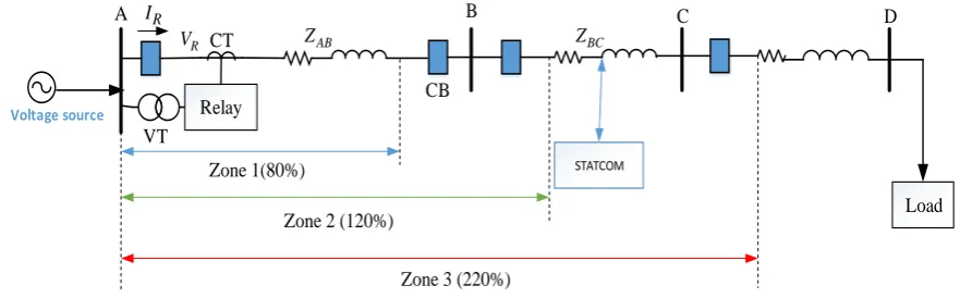
46
secured way of relaying operation in the protective system [4]. A numerous study were made for
47
location of fault in transmission lines in the literature, only some of the study involves effect of
48
FACTS compensated line and other fails to consider their effects [5-10]. The problem of over-reach
49
and under reach conditions due to the injection and absorption of reactive power by STATCOM into
50
the system leads to false tripping of relay [11]. Therefore, identification of fault in the presence of
51
FACTS device is a crucial issue in power system protection.
52
Distance relay based transmission line protection schemes were adapted for secure and reliable
53
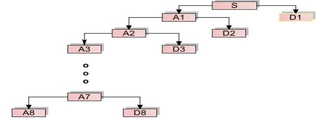
operation of system [12-14]. But, the presence of series/shunt FACTS device leads to mal-operation
54
of conventional relay to detect and locate the fault [15, 16]. Moreover, the fault signal is
55
non-stationary in nature and the analysis of such signal is a cumbersome process. Therefore,
56
researches proposed the numerical relays based on signal processing techniques namely Fourier
57
Transform (FT), Fast FT, discrete FT and short time FT that are extensively used in the initial stage
58
for analysis of fault signal. It is observed through rigorous analysis that FTs are not suitable for
59
locating time-varying fault transient signal and also the information on time of occurrence of
60
transients cannot be obtained. To cater this limitation S-transform based fault location were used for
61
locating the time and frequency information of fault signal. But it involves large number of
62
mathematical computation and calculation time that results in degrading the performance of
63
numerical relay [17-20].
64
The aforementioned drawback are overcome by the time-frequency based discrete wavelet
65
transform (DWT) approach and is broadly used for classification and location of faults, power
66
quality mitigation problems such as sag and swell in the system [21]. One of the major issues with
67
DWT is selection of mother wavelets and many works in the literature on analysis of power system
68
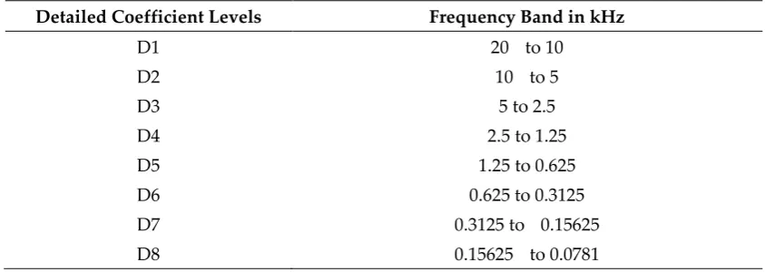
transients claimed that Daubechies 4 (db4) is best suited for fault analysis [22]. Because of fast
69
filtering with less processing time makes the DWT analysis than other methods for extracting the
70
features to train the Artificial Intelligence (AI) or machine learning (ML) classifiers in the proposed
71
work. Also, numerous computational intelligence classifiers were proposed for location of fault in
72
the system such as multilayer perceptron (MLP) neural network, support vector machine (SVM),
73
fuzzy logic, particle swarm optimization(PSO) and so on. The ANN and SVM classifiers consume
74
large time for training and the efficacy of fuzzy depends on rules framed by the expertise [6, 7, 13 23,
75
24.]. Also, many different methods of classifier are proposed in the literature ranging from heuristic
76
rule of thumb to formal mathematics [24]. Despite of all, the proposed work uses a simple, efficient
77
and sensitive type of probabilistic neural network based Naive Bayes (NB) approach for selection of
78
features to classify the type of fault in the system.
79
The remainder of the paper is organized as follows: Section 2 deals with the system model
80
studied and section 3 portrays the proposed method of fault classifications with detailed explanation
81
about extraction of features using DWT analysis. Section 4 describes the MLP neural network and
82
probabilistic network based classifiers such as Bayes and NB method to classify the fault occurs in
83
the system. Section 5 presents the results and discussion of proposed work of fault classification with
84
conclusion and future work made in the last part of the paper.
85
2. System Model Studied
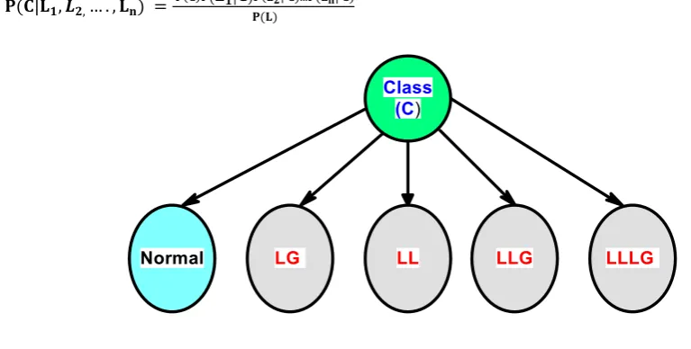
86
To validate the proposed method of fault detection scheme, it is necessary to acquire the field
87
data from the real time power system network. As the real time data acquisition is quite tedious and
88
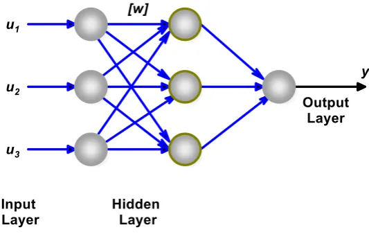
cumbersome process. Therefore, the system under study for fault application considers a real time
89
Libya power system data for simulation and the possibility of occurrence of numerous faults are
90
simulated using Mat lab/Simulink. Figure 1 depicts the shunt STATCOM compensated power
91
system model and the parameters for simulation are as follows: Generator rating – 300 MVA, 400kV,
92
load rating of 260 MVA. The detailed explanation of simulation parameters and STATCOM are
94
presented in [11]. The dataset for training of neural networks (NN) are obtained by introducing the
95
various fault considering effect of fault resistance and with/without STATCOM at different locations
96
like 100km, 200km and 300 km of mid-point compensated power system.
97
Relay CT
VT R I
A B
AB
Z ZBC C
Zone 1(80%)
Zone 2 (120%)
Zone 3 (220%)
R
V
CB
D
Load
Voltage source
STATCOM
98
Figure 1. Libya Power System Model
99
The power system model is protected from fault by different zones of protection scheme Z1, Z2 and
100
Z3. Thus, the relay responds to various zones of protection and the trip signal is obtained from the
101
intelligence relaying scheme developed using a NB classifier. In the proposed work, the percentage
102
of distance protection relay by different zones such as Z1, Z2 and Z3 are assumed to be 80%, 120%
103
and 220% of total line length respectively. .
104
2. 1. Proposed Method of Fault Detection
105
This section presents the steps for detection of fault in power system using NB method of
106
classification. The detailed steps is illustrated in Figure 2 and also presented as follows:
107
Step-1 Data Acquisition - The shunt compensated power system model is simulated using Mat
108
lab/Simulink under various cases of disturbances and the current signal is obtained for extracting the
109
features to train the NN.
110
Step-2Feature Extraction– The data for training are obtained by sampling the current signal using
111
advanced signal processing techniques like DWT and the features such as standard deviation (SD)
112
and energy values are obtained for the system with and without shunt compensation to study the
113
effect of STATCOM compensation.
114
Step-3Training Phase– In this phase, the obtained SD and energy values are acquired for different
115
location of faults and various values of fault resistance.
116
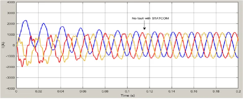
Step-4Fault detection– Here, the trained NN is tested for occurrence of different faults in the system
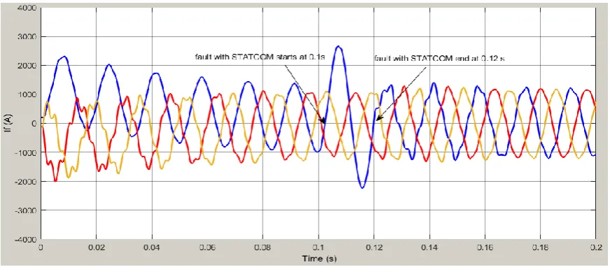
117
and this process repeats for every cycle of operation.
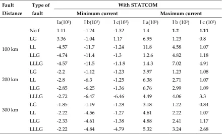
118
119
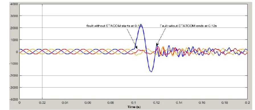
120
121
122
124
125
Figure 2. Proposed method of fault classification
126
3. Feature Extraction using Discrete Wavelet Transform
127
Wavelet transform (WT) have been widely used for analyzing the transient signal in ample
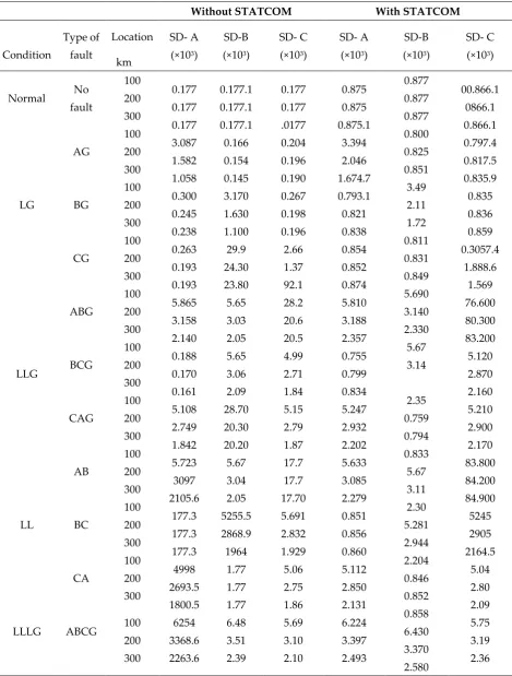
128
number of applications like mechanical vibrations, image processing and also electrical power
129
system fault detection. As wavelet analysis overcome the limitations of FT by localizing the fault
130
signal both in time and frequency domains. As Fourier analysis, does not provide information about
131
the time of occurrence of fault/disturbance in non-stationary current/voltage waveform of power
132
system. In general WT exists in two forms: continuous and discrete method. The later is extensively
133
used in the literature, due to its resolution and its applicability in real time. The detailed explanation
134
on application of WT in power system is discussed in [21,22].
135
DWT is a significant tool that analyzes the time varying, transient signal like faults by
136
decomposing it into an approximation (A) and detailed coefficients (D) through successive filtering
137
of high-pass and low-pass signal as depicted in Figure 3.
138
139
Figure 3. DWT Decomposition at eight levels
140
As the number of decomposition level increases, the DC noise present in the fault signal can be
141
suppressed. In this work, an mother wavelet of Db4 with 8-level is used to extract the features by
142
sampling the current signal of one cycle with the sampling frequency of 20 kHz and 333 samples per
143
cycle of current waveform. Among various mother wavelets exist in literature, Daubechies (Db4)
144
transients in low frequency sinusoidal signal. The bandwidth of each levels of decomposition is
146
presented in Table 1.
147
Table 1. Detailed Coefficient Levels Frequency Band kHz Detailed Coefficient Levels Frequency Band in kHz
D1 D2 D3
D4 D5
D6 D7
D8
20 to 10 10 to 5
5 to 2.5
2.5 to 1.25 1.25 to 0.625
0.625 to 0.3125 0.3125 to 0.15625
0.15625 to 0.0781
3.1 Feature Extractions
148
The main aim of feature extraction is to provide the significant information for the classifier to
149
classify the type of event through the features calculated using standard deviation (SD) and energy
150
values. The detailed information of this is discussed as follows,
151
3.1.1 Standard Deviation (SD)
152
The SD is statistical measure of how much variation or dispersion that exists in the original signal
153
and is defined in terms of wavelet coefficient as,
154
𝐒𝐃 = √{∑𝟖𝐢=𝟏(𝐀𝟖+𝐃𝐢)𝟐
𝐧 − (
∑𝟖𝐢=𝟏(𝐃𝟖+𝐃𝐢)
𝐧 )
𝟐
} (1)
155
where n represents the number of data samples.
156
3.1.2 Energy Value (E)
157
To test the effectiveness of the proposed classifier, this work uses another approach to calculate
158
features based on energy of the decomposed current signal. The spectral energy of the decomposed
159
signal can be obtained using Equation (2),
160
𝐄 = ∑𝐤𝐢=𝟏[|𝐃𝐢|𝟐] + |𝐀𝟖|𝟐
161
(2)
162
where k is the number of detailed coefficient levels. To calculate the features, a moving window of
163
one cycle of current wavelet coefficient is passed and the features are extracted for training the
164
classifiers [26].
165
4. Fault Classifiers
166
This section presents Bayesian based fault classifiers to identify and classify the type of fault that
167
occurs in the shunt compensated STATCOM devices. The comparative study is made with the
168
conventional MLP neural network for the system with and without STATCOM. Here in this work,
169
each fault that occurs in the system is considered as classes and the same is used for training neural
170
network. The assumed classes for classifications are: C1 -Normal, C2 -LG fault, C3 -LL fault, C4 -LLG
171
fault and C5 -LLLG fault. Moreover, the effectiveness of the method is also tested for occurrence of
172
174
4.1 Multi-Layer Perceptron (MLP) Network
175
Multi-Layer Perceptron (MLP) is the most widely used neural network for identification and
176
detection type of fault in power system in the literature. MLP is a supervised feed forward network,
177
as it requires learning the desired output to be classified. Figure 4 represents the MLP network that
178
consists of input (u1, u2 and u3), hidden and output layer.
179
180
Figure 4. MLP neural network
181
The output [y] of the network is weighted sum of input neurons and is defined as,
182
𝑦𝑖= 𝑊𝑖𝑜+ ∑𝑗∈𝑝𝑟𝑒𝑑(𝑖)(𝑊𝑖𝑗𝑎𝑗) (3)
183
where aj represents the output of previous layer neuron, Wij is the weight between ith and jth neuron and Wio is
184
input bias of neuron. In this work, the MLP network is trained using back propagation method and the detailed
185
explanation is presented in [27, 28].
186
4.2 Bayes and Naive Bayes Classifiers
187
The conventional MLP neural network minimizes the error of the system by adjusting the
188
weight of the network through small penalty factor that leads to overfitting. This is avoided for any
189
complex network through a principle approach called Bayes theorem by the Bayesian neural
190
network (BNN). BNN is invented by Judea Pearl in 1980s, a statistical based supervised classifier
191
that determines the variable to be classified in more relevant to the class by evaluating the
192
probability of how likely its occurrence in that class with the prior information that takes the form
193
prior probability density function [29]. Thus the Bayes theorem can be defined as
194
𝑷𝒐𝒔𝒕𝒆𝒓𝒊𝒐𝒓 𝒑𝒓𝒐𝒃𝒂𝒃𝒊𝒍𝒊𝒕𝒚 =𝑪𝒍𝒂𝒔𝒔 𝒑𝒓𝒊𝒐𝒓 𝒑𝒓𝒐𝒃𝒂𝒃𝒊𝒍𝒊𝒕𝒚∗𝒍𝒊𝒌𝒆𝒍𝒊𝒉𝒐𝒐𝒅
𝑷𝒓𝒆𝒅𝒊𝒄𝒕𝒐𝒓 𝒑𝒓𝒊𝒐𝒓 𝒑𝒓𝒐𝒃𝒂𝒃𝒊𝒍𝒊𝒕𝒚
195
(4)
196
The simplified form can be expressed as,
197
P(C|𝐋𝟏, 𝑳𝟐,… . , 𝐋𝐧) =
𝐏(𝐂)𝐏(𝐋𝟏,𝑳𝟐,….,𝐋𝐧| 𝐂).
𝐏(𝐋𝟏,𝑳𝟐,….,𝐋𝐧) (5)
198
𝑷(𝑪|𝑳) =𝑷(𝑪)𝑷(𝑳|𝑪)
𝑷(𝑳) (6)
199
Where P(C) is the class probability and P(L|C) represents the likelihood of datasets {L1, L2, …Ln} of
201
variables in class C=[C1, C2,…C5]. The classification problem can be defined as,
202
𝐚𝐫𝐠 [𝐦𝐚𝐱 [𝑷(𝑪|𝑳) =𝑷(𝑪)𝑷(𝑳|𝑪)
𝑷(𝑳) ]]
203
(7)
204
Here the attributed P(L) doesn’t vary with the class and can be assumed as constant and the above
205
equation is approximated as,
206
𝐚𝐫𝐠 [𝐦𝐚𝐱[𝑷(𝑪|𝑳) = 𝑷(𝑪)𝑷(𝑳|𝑪)]]
207
(8)
208
The computation burden of BNN is increases as the number of likelihood term in the class raises
209
exponentially with the attributes L= {L1, L2, … Ln }. To overcome this limitation, all features in a class
210
are assumed to be independent that results in the Naive Bayes (NB) classifier that reduces the
211
number of parameter to be estimated from 2(2n-1) to 2n [25, 30, 31]. NB is a linear classifier that
212
divides the input data set into training and prediction step for identifying the type of class using
213
Bayes’ theorem. In training phase, the classifier determines the probability distribution pertaining to
214
the features of any given class is independent. During the prediction phase, classifier estimates the
215
posterior probability of test sample data belonging to respective class. Then, the method classifies
216
the samples based on maximum likelihood of posterior probability. NB classifier has been used
217
widely because of its simplicity, easy to implement accuracy and sound theoretical basis that
218
guarantees the optimized results. The probability function defined in (8), can be rewritten with the
219
assumption of independent feature as,
220
𝐏(𝐂|𝐋𝟏, 𝑳𝟐,… . , 𝐋𝐧) =
𝐏(𝐂)𝐏(𝐋𝟏|𝐂)𝐏(𝐋𝟐| 𝐂)...𝐏(𝐋𝐧| 𝐂)
𝐏(𝐋) (9)
221
222
Figure 5. NB classifier of proposed work
223
4.2.1 Performance Indices of classifier
224
Kappa Statistic (K) is the statistical measure of classifiers that compute the constancy among
225
the predicted type of fault and actual type of fault and is defined as follows,
226
𝐾 =𝑃(𝑂𝐹)−𝑃(𝐸𝐹)
(1−𝑃(𝐸𝐹)) (10)
227
where P(OF) is the probability of observed fault, P(EF) is the probability of predicted type of fault.
228
Mean Absolute Error (MAE)and Root Mean Square Error (RMSE) - MAE is the absolute mean of
230
error calculated between the predicted and observed value and is depicted as follows [21, 38, 39],
231
𝑀𝐴𝐸 =|∑𝑛𝑖=1(𝐸𝑃−𝐸𝑂)|
𝑛 (11)
232
RMSE is the square root of mean of variance, between the predicted and observed type of fault
233
detected by the classifiers and is given by,
234
𝑅𝑀𝑆𝐸 = √∑𝑛𝑖=1(𝐸𝑃−𝐸𝑂)2
𝑛 (12)
235
where EP is the predicted type of fault and EO is the expected type of fault.
236
237
5. Results and Discussion
238
This section describes the simulation of proposed probabilistic NB based classifier to classify the
239
fault and location of fault in transmission line. The effect of probabilistic classifier is studied for the
240
transmission line with and without compensations. The simulation is carried out for power system
241
model depicted in Figure 1 and various plausible faults such as LG, LL, LLG and LLLG fault in the
242
system considering the variation in fault resistances. The simulation is carried out for time period of
243
one cycle and the fault is applied during 0.1 to 0.12 s. Figure 6 and 7 depicts the three phase current
244
waveform of the system without and with STATCOM respectively. The minimum and maximum of
245
peak magnitude of three phase current signal are captured for the system with and without
246
compensation that are illustrated in Table 2 and 3. It is seen the magnitude of current signal increases
247
for the system with STATCOM device and the same is presented in the form waveform for case of
248
LG fault in the system with and without STATCOM are portrayed in Figures 10 and 11 respectively.
249
Then, the current signal obtained for various cases of fault are analyzed using db4 mother wavelet of
250
DWT analysis with eight level coefficients to extract the features such as SD and energy values for
251
training the classifiers. Figures 8 and 9 represent the DWT analysis of current waveform under
252
normal operation of the system without and with STATCOM respectively. In general, the
253
coefficients are high for the compensated system compare to the uncompensated system. Figures 12
254
and 13 portray the DWT analysis of LG fault current waveform considering without and with
255
STATCOM respectively. Also, it is observed that the coefficients of detailed coefficient is low when
256
fault occurs after the location of STATCOM (at 150 km) device. This effect is due to the STATCOM,
257
the system fault current reduces as the distance of fault increase from, the fault location point. Table
258
4 and 5 represents the extracted features (SD and energy values) for training the classifiers. The
259
trained classifiers are tested with the test data and the type of fault that occurs in the system is
260
detected by the classifiers. The performance of classifier for classification of various faults in the
261
system for cases with and without STATCOM using the features of SD and energy values are
262
presented as different cases as discussed in forthcoming subsections.
263
Figure 6. Three phase current waveform under normal condition without STATCOM compensation
265
266
267
Table 2. Normal and LG faults at Different Locations without STATCOM compensation
268
269
Without STATCOM Fault Distance Type offault Minimum current Maximum current
Ia (103) I b(103) I c(103) Ia(103) I b(103) I c(103)
No fault LG LL LLG LLLG LG LL LLG LLLG LG LL LLG LLLG -0.25 -2.57 -4.11 -4.19 -3.88 -1.23 -2.19 -2.1 -1.97 -0.78 -1560 -1.51 -1.31 -0.25 -0.34 -12.5 -12 -12 -0.27 -7.01 -6.78 -7.06 -0.294 -4.78 -4.85 -5.17 -0.25 -0.46 -0.25 -0.71 -12.4 -0.39 -0.25 -0.45 -7.16 -0.37 -0.25 -0.51 -4.97 0.25 6.95 12.6 1.34 1.52 3.67 7.06 7.56 8.32 2.49 4.93 5.08 5.72 0.25 0.28 4.05 4.3 6.76 0.19 2.16 2.34 3.78 0.185 1.47 1.62 2.62 0.25 0.25 0.25 0.65 4.3 0.18 0.25 0.38 2.82 0.19 0.25 0.37 2.16 100 km 200 km 300 km
270
Table 3. Normal and SLG faults at Different Locations with STATCOM compensation
271
Fault Distance Type of fault With STATCOMMinimum current Maximum current
Ia(103) I b(103) I c(103) I a(103) I b (103) I c (103)
272
273
Figure 7. Three phase current waveform under normal condition with midpoint compensation
274
275
Figure 8. DWT analysis of Phase A under normal condition without compensation
277
278
279
Figure 9. DWT analysis of Phase A under normal condition with STATCOM compensation
280
Figure 10.Three phase current during LG fault in Phase A without compensation
282
283
Figure 11. Three phase current during LG fault in Phase A with compensation
284
285
287
Table 4. SD based feature values for classification
288
Without STATCOM With STATCOM
Condition
Type of
fault
Location SD- A
(×103)
SD-B
(×103)
SD- C
(×103)
SD- A
(×103)
SD-B
(×103)
SD- C
(×103) km
Normal No
fault 100 200 300 0.177 0.177 0.177 3.087 1.582 1.058 0.300 0.245 0.238 0.263 0.193 0.193 5.865 3.158 2.140 0.188 0.170 0.161 5.108 2.749 1.842 5.723 3097 2105.6 177.3 177.3 177.3 4998 2693.5 1800.5 6254 3368.6 2263.6 0.177.1 0.177.1 0.177.1 0.166 0.154 0.145 3.170 1.630 1.100 29.9 24.30 23.80 5.65 3.03 2.05 5.65 3.06 2.09 28.70 20.30 20.20 5.67 3.04 2.05 5255.5 2868.9 1964 1.77 1.77 1.77 6.48 3.51 2.39 0.177 0.177 .0177 0.204 0.196 0.190 0.267 0.198 0.196 2.66 1.37 92.1 28.2 20.6 20.5 4.99 2.71 1.84 5.15 2.79 1.87 17.7 17.7 17.70 5.691 2.832 1.929 5.06 2.75 1.86 5.69 3.10 2.10 0.875 0.875 0.875.1 3.394 2.046 1.674.7 0.793.1 0.821 0.838 0.854 0.852 0.874 5.810 3.188 2.357 0.755 0.799 0.834 5.247 2.932 2.202 5.633 3.085 2.279 0.851 0.856 0.860 5.112 2.850 2.131 6.224 3.397 2.493 0.877 0.877 0.877 0.800 0.825 0.851 3.49 2.11 1.72 0.811 0.831 0.849 5.690 3.140 2.330 5.67 3.14 2.35 0.759 0.794 0.833 5.67 3.11 2.30 5.281 2.944 2.204 0.846 0.852 0.858 6.430 3.370 2.580 00.866.1 0866.1 0.866.1 0.797.4 0.817.5 0.835.9 0.835 0.836 0.859 0.3057.4 1.888.6 1.569 76.600 80.300 83.200 5.120 2.870 2.160 5.210 2.900 2.170 83.800 84.200 84.900 5245 2905 2164.5 5.04 2.80 2.09 5.75 3.19 2.36 LG AG 100 200 300 BG 100 200 300 CG 100 200 300 LLG ABG 100 200 300 BCG 100 200 300 CAG 100 200 300 LL AB 100 200 300 BC 100 200 300 CA 100 200 300
LLLG ABCG 100
200 300
289
291
Table 5. Energy based feature values for classification
292
Without STATCOM With STATCOM
Condition Type of fault
Location Km
E- A (×108)
E-B
(×10
8)
E- C
(×10
8)
E-A
(×10
8)
E- B
(×10
8)
E-C
(×10
8)
Normal No
fault 100 200 300 100 200 300 100 200 300 100 200 300 100 200 300 100 200 300 100 200 300 100 200 300 100 200 300 100 200 300 100 200 300 1.25 1.25 1.25 96.4 25.9 12 1.64 1.44 1.5 1.39 1.33 1.18 3.01.0 87.1 41.8 1.36 1.2 1.18 318 94.6 41.6 255 74.7 35.6 1.24 1.24 1.24 308 91.5 40.50 42.5 125 57.5 0.49 0.49 0.49 0.56 0.56 0.51 57.1 15.3 7.08 0.76 0.6 0.63 223 65 30.4 184 54.6 25 0.73 0.51 0.52 254 73.9 35 174 53 23.5 0.5 0.49 0.49 241 70.5 33.3 0.4 0.4 0.4 0.51 0.51 0.46 0.51 0.41 0.37 72.9 18.8 8.47 0.71 0.5 0.45 179 53.4 22.7 313 93 41.2 4.05 0.4 0.4 169 50.2 22.3 312 93.4 41.3 315 94.7 40.7 22.7 22.7 22.7 128 56.5 42.7 21.3 25.8 22.3 21.7 21.2 22.1 307 105 63.8 20.8 21.3 22.1 326 106 66.9 265 92.6 56.8 22.4 22.4 22.4 314 103 65.5 414 1.30E+10 76.6 6.26 6.26 6.26 5.36 5.62 5.85 70.7 27.5 18.8 5.74 6.22 6.11 214 64 34.3 185 58.1 32.80 5.17 5.09 5.53 234 68.3 35.8 170 49.5 30.2 5.8 5.87 5.98 236 71.9 38.6 13.1 13.1 13.1 11.4 12.1 12.3 13.2 12.3 13 97.1 38.6 28.8 11.3 12.8 13.6 200 670 44.4 305 94.9 56.5 12.8 12.9 12.9 18.6 62.4 40.8 300 91.7 54.3 315 97 5.91 LG AG BG CG LLG ABG BCG CAG LL AB BC CA
LLLG ABCG
293
294
296
297
Figure 13. DWT analysis of Phase A during LG fault with compensation
298
Table 6. Confusion Matrix for Classification
299
Classes C1 C2 C3 C4 C5 System State
C1 C2 C3
C4 C5
1 0 0
0 0
0 1 0
0 0
0 0 1
0 0
0 0 0
1 0
0 0 0
0 1
Normal LG LLG
LL LLLG
300
Case-1: In this study, the transmission fault classification and identification in a transmission
301
different state of the system such as Normal, LG, LLG, LL and LLLG fault. Here, the fault in the
303
system is classified using the SD values obtained by the DWT analysis for different types of fault
304
occurring at the distance of 100 km, 200km and 300 km of an overhead transmission line is given in
305
Table 4. Then these data’s are used for training the neural network and the classification results
306
obtained are presented in the Table 7. The result shows that the proposed Naive Bayes (NB) method
307
of classifier is more accurate compared to the MLP and Bayes method of classification. Moreover, the
308
% misclassification rate of the proposed method is 0%, whereas the rate is 20% and 80 % for MLP
309
and Bayes approach of classification respectively. The MLP method of classification fails to detect
310
the LLG type of fault and on the other hand, the Bayes method fails to classify all type of fault and
311
whose performance is inferior compared to other methods. It is inferred from the Fig.. and Table..
312
that the NB classifier is the mostsignificant method, to classify the various type of fault in the system
313
compared to all other methods.
314
Case-2: Here in this study, the classification and identification offault is done without STATCOM as
315
like case-1. But in this case, instead of SD values the energy values obtained from DWT analysis for
316
different types of faults occurring at various distances of 100 km, 200 km and 300 km has been taken
317
for the training the network and which is illustrated in the Table5. The results obtained reveals that
318
NB method of classification is better than the other two methods such as MLP and Bayes classifiers.
319
Figure 14 represents the % accuracy rate of the proposed method is 100%, whereas is 60 % and 20 %
320
for MLP and Bayes network respectively. The MLP method of classification fails to detect LG and
321
LLG faults whilst Bayes classifier unable to detect all type of faults. It is seen that the propounded
322
NB has 0% misclassification rate, the MLP has 40% and Bayes method has 80% of misclassification
323
rate as depicted in Table 7.
324
Case-3: This case is similar to case-1, but in this study the STATCOM is connected at the midpoint of
325
the transmission line and the occurrence of faults at different location such as 100 km, 200 km and
326
300 km are studied. The SD values obtained are used to train the network as like the case-1 and the
327
results for classification are shown in Table 4. It is observed from the results that the proposed NB
328
classifier performance is more predominant in terms of accuracy and % misclassification rate
329
compared to the MLP and Bayes method of classification and is shown in Figure 14. The Bayes
330
method fails to identify all type of fault expect when the system is operating in normal condition and
331
MLP method fails to detect the LLG type of fault as like case-1. It is inferred from the results, both
332
the MLP and Bayes classifier performance is same for transmission line involving with and without
333
STATCOM and the proffered NB method classifier outperforms compared to these approaches.
334
Table7.ClassifiersAccuracy andMisclassification Rate
335
Accuracy Rate Misclassification Rate
Cases MLP Bayes Naïve Bayes
MLP Bayes Naive Bayes
% Rate Type of faul
Rate Type of Fault
Rate Type of Fault
Case-1
Case-2
Case-3
Case-4 80
60
80
100
20
20
20
20
100
100
100
100
2
40
20
0
C3
C2-C3
C3
0
80
80
80
80
C2-C5
C2-C5
C2-C5
C2-C5 0
0
0
0
0
0
0
Case-4: This case is analogous to case-2 with the incorporation of STATCOM connected at the
336
midpoint of the transmission line for supporting the reactive power and to improve the voltage
337
profile of the system performance. In this context, the energy values obtained from DWT analysis for
338
different types of faults at various distances of 100 km, 200 km and 300 km has been used for training
339
the network and which is portrayed in Table 5. Figure 14 represents the proposed NB classifier is
340
very efficient compared to the MLP and Bayes method. The % accuracy of NB and MLP are 100%
341
MLP, butthe Bayes method is only 20 % accurate. On the flipside, the % misclassification rate is 0%
342
for NB and MLP method and it is 80% for Bayes approach. It is deduced from the results, the
343
proffered NB classifier gives accurate results for all cases and its performance is significantly
344
predominant than the MLP and Bayes method as depicted in Table 7.
345
346
Figure 14. Comparision of Accuracy rate of classifiers
347
5.1 Performance Evaluation of Classifiers
348
The robustness of the classifier are evaluated by various performance indices such as Kappa
349
Statistics (KS), Mean Absolute Error (MAE), Root Mean Square Error (RMSE), Percentage Relative
350
Absolute Error (% MAE) and Percentage Root Relative Square Error (%RRSE) for classifiers namely
351
Bayes, MLP and NB approach. Firstly, the KS index for various classifier is presented in Table 8 and
352
Figure 15. The result shows that the indices is ‘1’ for the proposed NB classifier for all the cases and
353
the values lies in the range of 0.5-1 for MLP classifier (for various cases) and is almost ‘0’ for Bayes
354
method of classification. It is inferred from the KS index, the proffered method of classifier
355
outperforms for various cases compared to the other classifiers. Secondly, the MAE is less than 0.1
356
for the proposed classifier whereas the value lies in the range of 0.1-0.3 for MLP method and it is
357
greater than 0.3 for Bayes approach under various cases. Moreover, the RMSE is also less than 0.1 for
358
the NB method and the value lies in the range of 0.2-0.4 for MLP and it is almost 0.4 for Bayes
359
classifier for case-1 to case-4. It is seen that the indices such as MAE and RMSE are comparatively
360
very low as shown in Figsures 16 and 17 for the intended NB method of classifier than other
361
approaches presented, proves that the proposed classifier is more robust and efficient.
362
Lastly, the % RAE and %RRSE is proven to be significantly less for the propounded NB method
363
compared to MLP and Bayes classifier as depicted in Table 9 and Figure 18. It is observed the results
364
outperforms for all the cases by the NB approach rather than the MLP and Bayes classifier method.
365
366
0 20 40 60 80 100
Case 1
Case2
Case3
Case4
Accuracy Rate
Tabl 8. Performance comparison of various Classifiers
367
368
369
Figure 15. Kappa Statics comparison of various classifiers
370
371
Figure 16. MAE comparison of various classifiers
372
MLP Bayes
Navie Bayes
0 0.2 0.4 0.6 0.8 1
Case 1
Case2
Case3
Case4
Kappa Statistics
MLP Bayes Navie Bayes
0 0.05 0.1 0.15 0.2 0.25 0.3 0.35
Case 1
Case2
Case3
Case4
MAE
MLP Bayes Navie Bayes
Kappa Statistics MAE RMSE
MLP Bayes
Naive
Bayes MLP Bayes
Naive
Bayes MLP Bayes
Naive
Bayes
Case-1 Case-2 Case-3
Case-4
0.75 0.5 0.75
1
0 0 0
0
1 1 1
1
0.1596 0.2012 0.172
0.1551
0.32 0.32 0.32
0.32
0.0251 0 0.033
0
0.2369 0.2929 0.248
0.2276
0.4 0.4 0.4
0.4
0.0888 0 0.0979
373
Figure 17. RMSE comparison of various classifiers
374
375
376
Figure 18. %RAE comparison of various classifiers
377
378
Table 9. %RAE and %RRSE comparison of various classifiers
379
Cases
%RAE %RRSE
MLP Bayes Naive Bayes MLP Bayes Naive Bayes
Case-1
Case-2 Case-3
Case-4
49.89
62.8627 53.7439
48.4605
100
100 100
100
7.85
0 10.2998
0
59.23
73.2233 62.0026
56.8981
100
100 100
100
22.21
0 24.46
0
380
381
382
0 0.05 0.1 0.15 0.2 0.25 0.3 0.35 0.4
Case 1
Case2
Case3
Case4
RMSE
MLP Bayes Navie Bayes
0 20 40 60 80 100 120
MLP
Bayes
Navie
Bayes
MLP
Bayes
Navie
Bayes
%RAE
%RRSE
Relative Error
6. Conclusion
383
This paper presents a novel probabilistic based Navie Bayes approach to locate the fault in shunt
384
STATCOM compensated transmission line. In this work, a high voltage power system model of 400
385
kV has been simulated using MATLAB/Simulink and various faults such as LG, LL, DLG and LLLG
386
are applied. The current waveform obtained under different cases of normal and fault cases are
387
analyzed using DWT to extract the features for locating the type of fault. The fault current signal are
388
sampled with different band of frequencies that depicts 1st, 2nd, 3rd, 4th, 5th, 6th , 7th and 8th level
389
of detailed coefficient and its approximation coefficient at 8th level. The SD and Energy values have
390
been obtained for different faults with various fault resistance. The obtained features are used to
391
train the classifiers to classify the type of fault. The results obtained showed that the proposed NB
392
classifier outperforms with 100% accuracy rate in the case of with and without STATCOM. On the
393
flipside, the MLP method gives an average accuracy rate of 80% with Bayes of 20%. It also inferred
394
from the performance indices such as kappa statistics, MAE, %RAE and %RRSE, the proffered NB
395
approach gives the predominant result compared to the MLP and Bayes classifier method.
396
Author Contributions: E.A. and M.L.O proposed the main idea and performs the simulation of the work; V.V
397
and N.I.A.W provided sources and assisted to write paper; proof reading and final drafting was done by I.A
398
and H.H.
399
Funding: This research received no external funding
400
Acknowledgment: The authors are thankful to Center for Advanced Lightning Power and Energy Research
401
(ALPER) and Universiti Putra Malaysia to carry out this research.
402
Conflicts of Interest: The authors declare no conflict of interest.
403
References
404
1. Singh, A.R.; Patne, N.R.; Kale, V.S. Synchronized measurement based an adaptive distance relaying scheme for
405
STATCOM compensated transmission line. Meas. J. Int. Meas. Confed.2018, 116, 96–105.
406
2. Mirzaei, M.; Vahidi, B.; Hosseinian, S.H. Accurate fault location and faulted section determination based on deep
407
learning for a parallel-compensated three-terminal transmission line. IET Gener. Transm. Distrib.2019, 13,
408
2770–2778.
409
3. Ghazizadeh-Ahsaee, M.; Sadeh, J. Accurate fault location algorithm for transmission lines in the presence of
410
shunt-connected flexible AC transmission system devices. IET Gener. Transm. Distrib.2012, 6, 247.
411
4. Mishra, S.K.; Tripathy, L.N.; Swain, S.C. DWT approach based differential relaying scheme for single circuit and
412
double circuit transmission line protection including STATCOM. Ain Shams Eng. J.2019, 10, 93–102.
413
5. Chen, K.; Huang, C.; He, J. Fault detection, classification and location for transmission lines and distribution systems:
414
a review on the methods. High Volt.2016, 1, 25–33.
415
6. Veerasamy, V.; Abdul Wahab, N.I.; Ramachandran, R.; Thirumeni, M.; Subramanian, C.; Othman, M.L.; Hizam, H.
416
High-impedance fault detection in medium-voltage distribution network using computational intelligence-based
417
classifiers. Neural Comput. Appl.2019, 0123456789.
418
7. Veerasamy, V.; Abdul Wahab, N.I.; Ramachandran, R.; Mansoor, M.; Thirumeni, M.; Othman, M.L. High impedance
419
fault detection in medium voltage distribution network using discrete wavelet transform and adaptive neuro-fuzzy
420
inference system. Energies2018, 11.
421
8. Gupta, O.H.; Tripathy, M. An innovative pilot relaying scheme for shunt-compensated line. IEEE Trans. Power Deliv.
422
2015, 30, 1439–1448.
423
9. Mehrjerdi, H.; Ghorbani, A. Adaptive algorithm for transmission line protection in the presence of UPFC. Int. J. Electr.
424
Power Energy Syst.2017, 91, 10–19.
10. Albasri, F.A.; Sidhu, T.S.; Varma, R.K. Performance comparison of distance protection schemes for shunt-FACTS
426
compensated transmission lines. IEEE Trans. Power Deliv.2007, 22, 2116–2125.
427
11. Aker, E.E.; Othman, M.L.; Aris, I.; Wahab, N.I.A.; Hizam, H.; Emmanuel, O. Adverse impact of STATCOM on the
428
performance of distance relay. Indones. J. Electr. Eng. Comput. Sci.2017, 6, 528–536.
429
12. Othman, M.L.; Aris, I.; Wahab, N.I.A. Modeling and simulation of the industrial numerical distance relay aimed at
430
knowledge discovery in resident event reporting. Simulation2014, 90, 660–686.
431
13. Othman, M.L.; Aris, I.; Othman, M.R.; Osman, H. Rough-Set-and-Genetic-Algorithm based data mining and Rule
432
Quality Measure to hypothesize distance protective relay operation characteristics from relay event report. Int. J. Electr.
433
Power Energy Syst.2011, 33, 1437–1456.
434
14. Othman, M.L.; Aris, I.; Othman, M.R.; Osman, H. Rough-Set-based timing characteristic analyses of distance
435
protective relay. Appl. Soft Comput. J.2012, 12, 2053–2062.
436
15. Hussain, S.; Osman, A.H. Fault location on series and shunt compensated lines using unsynchronized measurements.
437
Electr. Power Syst. Res.2014, 116, 166–173.
438
16. Kumar, B.; Yadav, A.; Pazoki, M. Impedance differential plane for fault detection and faulty phase identification of
439
FACTS compensated transmission line. Int. Trans. Electr. Energy Syst.2019, 29, 1–21.
440
17. Megahed, A.I.; Moussa, A.M.; Bayoumy, A.E. Usage of wavelet transform in the protection of series-compensated
441
transmission lines. IEEE Trans. Power Deliv.2006, 21, 1213–1221.
442
18. Patel, B. A new FDOST entropy based intelligent digital relaying for detection, classification and localization of faults
443
on the hybrid transmission line. Electr. Power Syst. Res.2018, 157, 39–47.
444
19. Krishnanand, K.R.; Dash, P.K. A new real-time fast discrete S-transform for cross-differential protection of
445
shunt-compensated power systems. IEEE Trans. Power Deliv.2013, 28, 402–410.
446
20. Dash, P.K.; Das, S.; Moirangthem, J. Distance protection of shunt compensated transmission line using a sparse
447
S-transform. IET Gener. Transm. Distrib.2015, 9, 1264–1274.
448
21. Wilkinson, W.A.; Cox, M.D. Discrete wavelet analysis of power system transients. IEEE Trans. Power Syst.1996, 11,
449
2038–2044.
450
22. Osman, A.H.; Malik, O.P. Protection of Parallel Transmission Lines Using Wavelet Transform. IEEE Trans. Power
451
Deliv.2004, 19, 49–55.
452
23. Devasahayam, V.; Veluchamy, M. An enhanced ACO and PSO based fault identification and rectification approaches
453
for FACTS devices. Int. Trans. Electr. Energy Syst.2017, 27, 1–11.
454
24. Dash, P.K.; Samantaray, S.R.; Panda, G. Fault classification and section identification of an advanced
455
series-compensated transmission line using support vector machine. IEEE Trans. Power Deliv.2007, 22, 67–73.
456
25. Zhang, N.; Wu, L.; Yang, J.; Guan, Y. Naive bayes bearing fault diagnosis based on enhanced independence of data.
457
Sensors (Switzerland)2018, 18, 1–17.
458
26. Hindarto; Muntasa, A. Wavelet sub-band energy for feature extraction of electro encephalo graph (EEG) signals. J.
459
Eng. Sci. Technol.2019, 14, 578–588.
460
27. Patil, K.; Jadhav, N. Multi-Layer Perceptron Classifier and Paillier Encryption Scheme for Friend Recommendation
461
System. 2017 Int. Conf. Comput. Commun. Control Autom. ICCUBEA 20172018, 1–5.
462
28. Deep, K.; Nagar, A.; Pant, M.; Bansal, J.C. Proceedings of the Second International Conference on Soft Computing for
463
Problem Solving (SocProS 2012), December 28-30, 2012; 2014; Vol. 236; ISBN 978-81-322-1601-8.
464
29. Youn, E.; Jeong, M.K. Class dependent feature scaling method using naive Bayes classifier for text datamining.
465
Pattern Recognit. Lett.2009, 30, 477–485.
466
30. Addin, O.; Sapuan, S.M.; Mahdi, E.; Othman, M. A Naïve-Bayes classifier for damage detection in engineering
467
materials. Mater. Des.2007, 28, 2379–2386.
31. Muralidharan, V.; Sugumaran, V. A comparative study of Naïve Bayes classifier and Bayes net classifier for fault
469
diagnosis of monoblock centrifugal pump using wavelet analysis. Appl. Soft Comput. J.2012, 12, 2023–2029.