Optimization of Digital Transfer Textile Printing Process
using Multi-Objective Function Analysis
Dong Won Jeon1, Sungmin Kim, PhD2, In Hwan Sul3, Chang Kyu Park1
1
Department of Organic and Nano System Engineering, Konkuk University, Seoul KOREA
2
Department of Textiles, Merchandising, and Fashion Design, Seoul National University, Seoul KOREA
3
Department of Materials Design Engineering, Kumoh National Institute of Technology, Gumi KOREA
Correspondence to:
Chang Kyu Park email: [email protected]
ABSTRACT
Digital textile printing (DTP) is widely used because it is more efficient and simpler than conventional textile printing methods. Digital transfer textile printing (DTTP) is one of the most efficient and simplest DTP methods. In this study, the optimum process conditions for DTTP have been investigated, to minimize the distortion of printed images and maximize the color reproducibility. First, a novel measurement method for fabric shrinkage and image distortion was developed. Then 9 characteristic values were defined and a series of experiments were designed and performed using the Taguchi method. Finally, two different multiple-characteristic value analyses were performed on the results. In one method, 9 characteristic values were converted into a single value. In the other method, the characteristic values were divided into 3 groups for analysis. Finally, results from the two methods were compared to determine which method was more suitable.
INTRODUCTION
Until recently, the textile industry has been dependent upon the mass production of limited types of goods. However, a new concept for mass customization has evolved to meet the demands of modern customers. Although the future of mass customization is very promising, it cannot compete with mass production in terms of price because conventional dyeing processes are too expensive. Therefore, DTP (Digital Textile Printing) is considered to be one of the most
important technologies to successful
commercialization of mass customization [1]. Since DTP does not require costly manual processes such as color separation and silk screening, it dramatically shortens the time for dyeing or printing. Another advantage of DTP is that there is no limit to the complexity of design, a major limitation of conventional silk screen printing.
There are two major methods in DTP. In one method, images are directly printed on the fabric, whereas in the other method, images are printed on a paper and then transferred to the fabric. The latter is called DTTP (Digital Transfer Textile Printing) and it is widely used because it is easier to print on paper than on a fabric because the fabric has poor dimensional stability. Since there is no specific method to evaluate the dimensional stability of printed fabric during the DTTP process, a novel evaluation method has been developed in this study through modification of existing techniques.
To determine the optimum conditions for the DTTP process, the Taguchi method was used [2-5]. It has been widely used in many research fields, but only in a few applications in garment manufacturing. Yoon et al. used an expert system with the Taguchi method to find the optimum condition for a fusing process to maximize the delamination strength of fusible interlinings [6]. Park et al. tried to find the optimum sewing conditions to minimize seam pucker using the Taguchi method [7]. Yuen et al tried to find the factors influencing color yield of an ink-jet printed cotton fabric using the Taguchi method [8].
DEFINITION OF CHARACTERISTIC VALUES Skewness
A square test image was printed on the fabric to measure the skewness of fabric after post processing as shown in Figure 1(a). Skewness was defined as Eq. (1) and was evaluated by three methods. One was the measurement of the magnitude of four corner angles of the square represented by circle marks. Another was the measurement of intersecting angles between the top side of the square and the three lines drawn parallel to the wale direction through two triangle marks. The third was the measurement of intersecting angles between lines drawn parallel to the wale and course directions on four diamond marks. All the measurements were made after 4 hours of conditioning under standard atmospheric temperature and humidity according to ISO139. To prevent deformation of fabric by external forces, heavy weights were applied to both ends of fabric during all measurements in the wale and course directions.
,
100
10 0
n
s
S
s
n
i i
i i i i
∑
=
=
×
−
=
θ
θ
θ
(1)
3 2, 1, for type 4 , 3 , 4
s postproces after
Angle
s postproces before
Angle
s postproces after
rate distortion Average
s postproces after
rate distortion th
,
0
= = = = =
n S
i s where i
θ θ
Dimensional Stability
To measure the dimensional stability of a fabric after dry heating, a novel evaluation method has been developed as an alternative to the conventional ISO 5077:2007 method for measuring dimensional stability after washing and drying. In this method, a 30cm x 30cm square image was printed as shown in
Figure 1(b) and the length of each side was measured along the wale and course directions. Fabric specimens were dry heated according to ISO139 and
conditioned approximately 4 hours before
measurement. To prevent deformation of the specimen during the measurement, heavy weights were applied on both ends of a specimen. The deformation rate was calculated in course and wale directions respectively using Eq. (2).
100
0
0
−
×
=
l
l
l
S
(2)s postproces after
square the of side a of Length
s postproces before
square the of side a of Length
s postproces after
rate n Deformatio
,
0
= = =
l l S where
FIGURE 1. Images for measurement (a) Skewness (b) Dimensional Stability.
Color Strength
Apparent color strength (K/S) was measured using a Color-Eye 3100 CCM (Color coordination measurement) apparatus (Macbeth, USA). The entire surface of each specimen was measured thrice and four K/S values were measured in 400~700 nm range including cyan, magenta, yellow, and black [9].
PREPARATORY EXPERIMENT FOR TRANSFER PRINTING CONDITION
Experimental Design
Materials
Fabrics that were sensitive to distortion were chosen for skewness measurement. Fabrics made of spandex yarn the highest sensitivity in preparatory experiments and a polyester/spandex blended fabric DBR-WS36 was chosen.
Transfer Paper
Transfer paper was printed using an SC-S70610 printer (Epson, Japan) with 8 colors including cyan, magenta, yellow, black, light cyan, light magenta, orange, and grey. Images were prepared using Illustrator (Adobe, USA).
A total of 20 rows x 6 columns of 5cm x 5cm square images were printed in black color as the test image (Figure 2) in to evaluate the overall dimensional stability of the fabric.
Post Processing
FIGURE 2. Image for the measurement of fabric dimensional stability.
Factors and Levels
The factors and their levels used in this study are as shown in Table I. De facto standard temperature of 220oC and speed of 20 m/min were considered to be the base conditions. Temperature was varied in increments of 10oC and speeds were changed in increments 5 m/min. The upper limit of temperature was set to 225oC because excessive heat seemed to damage the fabric.
TABLE I. Factors and levels.
Temperature (℃)
225 225 225
220 220 220 220
210 210 210 210
200 200 200 200
Speed (m/in)
15 20 25
15 20 25 30
15 20 25 30
15 20 25 30
Results
The deformations in the wale and course directions were measured and analyzed using a t-test. No significant difference was observed across 6 consecutive grids. Therefore the dimension of test image was determined to be 30 cm. The heating drum used in post processing has the shape of a cylinder with center-bulged profile to maintain alignment of the fabric inside the machine. This shape exerts more pressure in the middle of the fabric, resulting in higher color reproducibility in that area. Therefore, only the images near the center of fabric were chosen for measurement in this study.
Fabric deformation was minimized a speed of 15 m/min. Therefore the speeds used were 10, 15, 20, and 25 m/min. The temperature interval of 10oC seemed to be too large for accurate measurement so the temperature increment was adjusted to 5oC.
MAIN EXPERIMENTAL DESIGN Factors and Levels
Four factors were chosen as shown in Table II,
including the type of transfer paper, heat treatment, postprocess temperature, and postprocess speed. The number of levels for each factor was 2, 2, 4, and 4.
TABLE II. Factors and levels.
Factor Symbol No. of
Levels Level
Postprocess Temperature
(℃)
A 4 AA1=210, A2= 215,
3=220, A4= 225
Postprocess Speed (m/min)
B 4 B1=10, B2= 15, B3= 20, B4=25
Heat
Treatment C 2 C1=Yes, C2=No
Paper Type
(g/m2) D 2 D1=58, D2= 90
Experimental Design
An L12(29) orthogonal array was used for
experimental design. The number of factors and their levels is shown in Table III.
TABLE III. L12(29) orthogonal array.
Exp.
No. 1 2 3 4 5 6 7 8 9
1 1 1 1 1 1 1 1 1 1
2 1 1 1 1 1 2 2 2 2
3 1 1 2 2 2 1 1 1 2
4 1 2 1 2 2 1 2 2 1
5 1 2 2 1 2 2 1 2 1
6 1 2 2 2 1 2 2 1 2
7 2 1 2 2 1 1 2 2 1
8 2 1 2 1 2 2 2 1 1
9 2 1 1 2 2 2 1 2 2
10 2 2 2 1 1 1 1 2 2
11 2 2 1 2 1 2 1 1 1
12 2 2 1 1 2 1 2 1 2
a b ab c ac bc ab
c d ad * The number in a cell means the level of a corresponding factor
After converting this into an L12(42x23) orthogonal
TABLE IV. L12(42x23) orthogonal array.
* The number in a cell means the level of a corresponding factor
Analysis Method
Taguchi Method
The Taguchi method is a robust design technique used to efficiently determine optimum experimental conditions [1,2,10]. Characteristic values are categorized as one of three types including nominal-is-best, smaller-the-better, and larger-the-better. The nominal-is-best type characteristic value has an optimum value when it becomes equal to the target value and used for length, weight, or thickness. The smaller-the-better type value has an optimum value when it becomes as small as possible and used for noise, wear, and defect ratio. The larger-the-better type value has an optimum value when it becomes as large as possible and used for strength, life, or efficiency [1]. In this study, the S/N (Signal to Noise) ratios of dimensional stability and skewness were regarded as smaller-the-better type values the K/S value was regarded as larger-the-better type value in optimizing of condition.
Grey Relation Analysis
Gray system theory was first proposed by Deng in 1982, which deals with systems with ambiguous and imperfect information. This theory has the advantage over other statistical analysis methods in that it does not assume any kind of statistical distribution to predict the behavior of the system of interest. In this method, normalized S/N ratios are represented by grey relational coefficients to be evaluated into grey relational grade. It should be noted that the relationship among the characteristic values is not considered in this method [3].
Desirability Function Analysis
In this method, S/N ratios are converted into desirability. The information of each characteristic value is reflected in it because the limit of each
characteristic value is considered during the conversion. The relationship among the characteristic values is not considered in this method either [3].
RESULTS AND DISCUSSION Taguchi Method
Dimensional Stability
Each of 12 experiments was repeated three times to obtain the S/N ratio. Since the dimensional stability was a smaller-the-better characteristic value, the S/N ratio was calculated using Eq. (3).
1
log
10
ratio)
/
(
1 2
−
=
∑
=
n
j ij
i
y
n
N
S
(3)point experiment an
in of count repeat
experiment th
of value stic characteri th
,
y n
i j
y where ij
= =
The S/N ratio at each experimental point is shown in
Table V.
TABLE V. S/N Ratio of dimensional stability.
The sum of squares of the error for a given column in the orthogonal array can be calculated using Eq. (4):
Sum of squares =
level
at values stic characteri of number
) level at values stic characteri of (sum
2
1 1
2
N y
i i
p
i i p
i
−
∑
∑
==
(4)
column in the levels of number
values stic characteri of
number total ,
= =
p N where
Contribution at each level is calculated using Eq. (5).
ratio S/N average Total -level each at ratio S/N Average
on
Contributi = (5)
In this study, factors with smaller sum of squares than that of the error term were pooled. For dimensional stability, factor A was pooled in the wale direction and all factors except B were pooled in the course direction.
Exp. No A B C E G
1 1 1 1 1 1
2 2 1 1 1 2
3 1 2 2 2 1
4 2 4 1 2 2
5 2 3 2 2 1
6 1 4 2 1 2
7 4 2 2 1 2
8 3 1 2 2 2
9 4 2 1 2 1
10 4 3 2 1 1
11 3 4 1 1 1
12 3 3 1 2 2
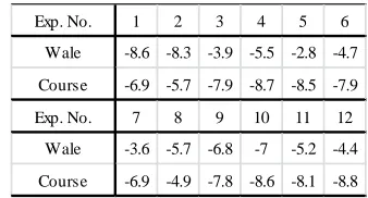
Exp. No. 1 2 3 4 5 6
Wale -8.6 -8.3 -3.9 -5.5 -2.8 -4.7 Course -6.9 -5.7 -7.9 -8.7 -8.5 -7.9
Exp. No. 7 8 9 10 11 12
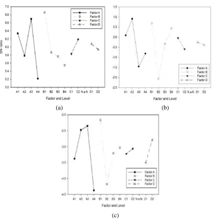
The average S/N ratio of each dimensional stability factor is shown in Figure 3.
FIGURE 3. S/N Ratio of dimensional stability (a) Wale direction (b) Course direction.
According to the analysis results, the optimum condition for the wale direction was A3 B3 C2 D2 and A3 B1 C2 D1 for the course direction. However, since all factors except B were pooled, the overall optimum condition was B1.
Skewness
Each of 12 experiments was repeated three times to determine the S/N ratio. The skewness was a smaller-the-better characteristic value. The S/N ratio for each experimental point is as shown in Table VI.
TABLE VI. S/N ratio of skewness.
Average S/N ratio of each factor for skewness is as shown in Figure 4.
FIGURE 4. S/N ratio of skewness (a) Type 1 (b) Type 2 (c) Type 3
According to the analysis results, the optimum condition for type 1 skewness was A3 B1 C2 D1. The optimum condition for type 2 skewness was A2 B1 C2 D1 but since factor D was pooled, the final condition was A2 B1 C2. The optimum condition for type 3 skewness was A1 B4 C2 D1 but since factors C and D were pooled, the final condition was A2 B1.
K/S
Each of 12 experiments was repeated three times to determine the S/N ratio. K/S was a larger-the-better characteristic value. The S/N ratio for each experimental point is as shown in Table VII.
TABLE VII. S/N ratio of K/S.
Factors A, C, and D were pooled for cyan. Factors C and D were pooled for other colors.
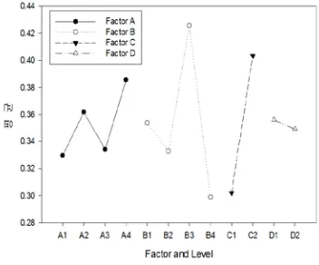
The average S/N ratio of each factor for K/S is shown in Figure 5.
(a)
(b)
Exp. No. 1 2 3 4 5 6
Type1 6.47 6.74 7.98 5.27 5.34 4.56 Type 2 3.46 -1.51 1.78 3.98 0.28 -4.97 Type 3 -2.97 -2.89 -3.14 -1.59 -2.95 -4.02
Exp. No. 7 8 9 10 11 12
Type1 5.85 7.36 3.77 6.03 6.8 5.93 Type 2 -6.29 0.12 -1.66 5.52 2.32 -6.8 Type 3 -3.92 -0.62 -5.47 -3.72 -3.48 -2.95
(a) (b)
(c)
Exp. No. 1 2 3 4 5 6
Cyan 14.9 14 16.3 16.9 16.5 16.5
Magenta 22.3 22.2 22.6 22.1 22.5 19.5 Yellow 23.6 23.5 23.6 23.2 23.5 20.3 Black 23.4 23.2 23.4 22.9 23.1 20.5
Exp.No. 7 8 9 10 11 12
Cyan 15.3 12.5 13.7 16.9 17.2 15.9
Magenta 22.6 21.7 22.3 23 21 22.3
FIGURE 5. S/N Ratio of K/S (a) Cyan (b) Magenta (c) Yellow (d) Black.
According to the the analysis results, the optimum condition for cyan was A4 B3 C1 D2 but since factors A, C, and D were pooled, the final condition was B3. For magenta, A4 B3 C1 D2 was the optimum condition but since factors C and D were pooled, the final condition was A4 B3. For yellow, the optimum condition was A4 B2 C1 D2 but since factor C was pooled, final the condition was A4 B3 D2. For black, the optimum condition was A4 B2 C1 D2 but since factors C and D were pooled, the final condition was A4 B3.
Multiple Characteristic Function Analysis
In this study, two types of multiple characteristic function analysis methods were used. In one method, 9 characteristic values were converted into a single value using a simple average and grey relation analysis. In the other method, 9 characteristic values were divided into 3 groups before simple average, grey relation analysis, and desirability function analysis. A more detailed explanation of these methods follows.
Calculation of Average
The average of 9 characteristic values was calculated using Eq. (6) with normalized S/N ratios.
min max
min
j j
j ij ij
SN
SN
SN
SN
u
−
−
=
(6)i j
SN
i j SN
where
j j
factor same in the value minimum the
having
point al experiment of
ratio S/N the
factor same in the value maximum the
having
point al experiment of
ratio S/N the ,
min max
= =
Calculated average values are shown in TableVIII. TABLE VIII. Average characteristic values.
Exp. No. 1 2 3 4 5 6
Average 0.62 0.59 0.74 0.64 0.66 0.27
Exp. No. 7 8 9 10 11 12
Average 0.62 0.66 0.41 0.69 0.55 0.56
A cause and effect diagram of the average calculation is as shown in Figure6.
FIGURE 6. Case and effect diagram of average calculation.
In this method, the optimum condition was A2 B3 C2 D2. The final condition was A2 B3 D2 after pooling factor C.
Grey Relation Analysis
S/N ratios were normalized using Eq. (6). The Grey relational coefficient representation of the normalized S/N ratio is calciulated using Eq. (7).
|
|
all
of
maximum
|
|
all
of
minimum
|
|
0 max
0 min
0
max max min
, 0
i i ij
ij ij ij
u
u
u
u
u
u
t
t
−
=
∆
=
−
∆
−
=
∆
∆
+
∆
∆
+
∆
=
ε
(7)
t is a coefficient to control the effect of design parameters and has a value between 0 and 1. Ten cases were analyzed with the value of t from 0 to 1 at intervals of 0.1.
(a) (b)
The gray relation grade was calculated by a weighted sum using Eq. (8) with calculated gray relational coefficients.
1
1 1 , 0∑
∑
= ==
=
n j j n j ij j iw
w
r
ε
(8)All wj were set to 1/9 in this study. The optimum
conditions obtained using gray relation analysis was A4 B3 C2 D1 with the t value of 0.1 from 0.7 and A2 B2 C2 D2 with the t value of 0.8 to 0.9.
Desirability Function Analysis
The desirability value was calculated using Eq. (9).
ij U j ij U j ij L j S L j U j L j ij ij L j ij ij SN SN d SN SN SN SN SN SN SN d SN SN d ≤ < < − − = ≤ = =1 0 (9) lue better va -the -larger for 1 log 10 ue better val -the -smaller for ) log( 10 ,..., 2 , 1 }, { max parameter shape , 2 2 1 − = − = = = = ≤ ≤ j L j j L j ij m i U j LSL SN USL SN n j SN SN s where Where j
USL and LSLjrefer to the standard upper and
lower limits of each characteristic value to set a valid range of experimental results [10].
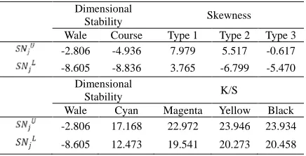
The minimum and maximum S/N ratios are shown in
Table IX.
TABLE IX. Upper and lower Limits of S/N ratio.
Dimensional
Stability Skewness
Wale Course Type 1 Type 2 Type 3 -2.806 -4.936 7.979 5.517 -0.617 -8.605 -8.836 3.765 -6.799 -5.470
Dimensional
Stability K/S
Wale Cyan Magenta Yellow Black -2.806 17.168 22.972 23.946 23.934 -8.605 12.473 19.541 20.273 20.458
Analysis was performed with s values of 0.5, 1, and 2. All data was converted into desirability values and unified into overall desirability values using a geometric average based on Eq. (10).
(
)
∑
==
×
×
×
=
n j j W W in W i W i overall iW
W
d
d
d
D
n 1 / 1 2 1 ,...
2 1 (10) ty desirabili th of weigth ,W j where j=Every Wjvalue was assumed to be 1 in this study. The
optimum condition obtained by desirability function analysis was A1 B2 C2 D2 regardless of the shape parameter.
Multiple Characteristic Function Analysis after Grouping
Nine characteristic values were divided into 3 groups. One group consisted of dimensional stability in the wale and course direction, a second group consisted of skewness 1, 2, and 3 and the third group consisted of the K/S values of cyan, magenta, yellow, and black. Grouped values were analyzed using the multiple characteristic function analysis method. The resulting three characteristic values were analyzed again using the same functions to calculate the final value.
Grey Relation Analysis
Grey relation analysis was performed to determine 3 characteristic values from each group. Those values were analyzed again to calculate the final value. S/N ratio was normalized using Eq. (6). The Grey relation coefficient was obtained using Eq. (7). The term t is a coefficient that controls the effects of design parameters and has a value between 0 and 1. Ten cases were analyzed with the value of t ranging from 0 to 1 at intervals of 0.1. The Grey relation grade was calculated by weighted sum using Eq. (8) with the calculated gray relational coefficients. Every Wj value
was assumed to be 1 in this study. The experimental condition that maximizes the grey relation coefficient is considered the optimum That one was A3 B1 C2 D2 in this study.
Desirability Function Analysis
into desirability values and an overall desirability value was calculated by geometric mean using Eq. (10). Secondary analysis was performed using these 3 overall desirability values. The optimum condition was A1 B2 C2 D2 regardless of the shape parameter.
Comparison of Expected Loss
Expected losses were compared between two analysis
methods. Experiments with minimum and
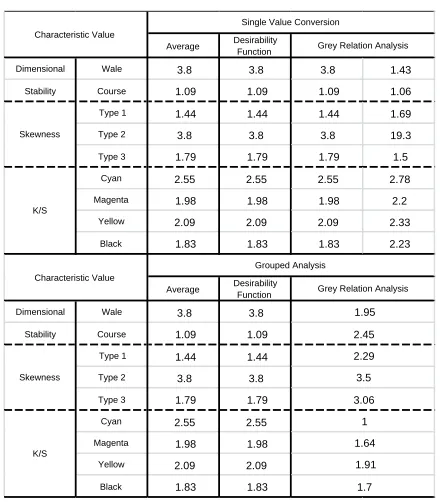
characteristic values were compared. The expected loss of each characteristic value is shown in Table X. The best results were obtained by using grey relation analysis with the single value conversion method. The largest improvement is found in skewness type 2. K/S values were improved as well. Dimensional stability showed the least improvement.
Results showed that the simple average method was unsuitable for accurate calculation. Simple averaging could not account for the complex variation of the data. Desirability function also seemed inappropriate it discarded too much data during the calculations. Grouping of characteristic values seemed minimally effective because the two-step function analysis could result in considerable errors during the calculation process.
CONCLUSION
In this study, the Taguchi method was used to determine the optimum processing conditions and maximize the reproducibility of DTTP. Four optimum conditions have been obtained for each characteristic value. A series of multi-object function analyses were performed to choose a single optimum condition among them by analyzing 9 characteristic values together. The optimum conditions determined by simple averaging were post process temperature (PPT) of 215 oC, post process speed (PPS) of 20 m/min and paper weight (PW) of 90g. Optimum conditions determined by desirability function analysis were PPT of 215oC and PPS of 20 m/min. Grey relation analysis resulted in two optimum conditions according to the classification coefficient. One was PPT of 225 oC, PPS of 20 m/min, and PW of 90g. The other was PPT of 215 oC, PPS of 20m/min and PW or 90g. After grouping the characteristic values, the simple average method resulted in the same condition mentioned above. Desirability function analysis resulted in optimum PPT of 215 oC and PPS of 20 m/min. Grey relation analysis resulted in optimum PPT of 220 oC, PPS of 10m/min, and PW of 90g.
By comparing the expected loss of all results above, grey relation analysis using the single characteristic value conversion method was shown to be the best method. That yielded an optimum PPT of 215oC, PPS of 20 m/min, and PW of 90g.
TABLE X. Comparison of expected loss.
ACKNOWLEDGEMENT
This paper was supported by Konkuk University in 2014.
REFERENCES
[1] Ujiie H., "Digital Printing of Textiles", Woodhead publishing, Cambridge, UK, 2006.
[2] Taguchi G., "Introduction to Quality
Engineering", Asian Productivity
Organization, Tokyo, Japan, 1986.
[3] Roy. R. K., "A Primer on the Taguchi Method", Society of Manufacturing Engineers, Dearborn, USA, 1990.
[4] Taguchi G., Chowdhury S,, and Taguchi S., "Robust Engineering", McGraw-Hill, New York, USA, 1999.
[5] Fowlkes W.Y. and Creveling , "Engineering Methods for Robust Product Design: Using Taguchi Methods in Technology and Product Development", Prentice Hall, New York, USA, 1995.
Average Desirability Function
Dimensional Wale 3.8 3.8 3.8 1.43
Stability Course 1.09 1.09 1.09 1.06
Type 1 1.44 1.44 1.44 1.69
Type 2 3.8 3.8 3.8 19.3
Type 3 1.79 1.79 1.79 1.5
Cyan 2.55 2.55 2.55 2.78
Magenta 1.98 1.98 1.98 2.2
Yellow 2.09 2.09 2.09 2.33
Black 1.83 1.83 1.83 2.23
Average Desirability Function
Dimensional Wale 3.8 3.8
Stability Course 1.09 1.09
Type 1 1.44 1.44
Type 2 3.8 3.8
Type 3 1.79 1.79
Cyan 2.55 2.55
Magenta 1.98 1.98
Yellow 2.09 2.09
Black 1.83 1.83
K/S
1
1.64
1.91
1.7 1.95
2.45
Skewness
2.29
3.5
3.06
Characteristic Value
Single Value Conversion
Grey Relation Analysis
Skewness
K/S
Characteristic Value
Grouped Analysis
[6] Yoon S. Y., Park C. K., Kim H. S., and Kim S., "Optimization of Fusing Process Conditions using the Taguchi Method", Textile Research Journal, 80(11), 2010, pp. 1016-1026.
[7] Park C. K. and Ha J. Y., "A Process for Optimizing Sewing Conditions to Minimize Seam Pucker using the Taguchi Method",
Textile Research Journal, 75(3), 2005, pp. 245-252.
[8] Yuen C. W. M., Ku S. K. A., Choi P. S. R., and Kan C. W., "Study of the Factors Influencing Color Yield of an Ink-jet Printed Cotton Fabric", Coloration Technology, 120(6), 2004, pp. 320-325.
[9] Das D. and Thakur R., "Taguchi Analysis of Fabric Shrinkage", Fibers and Polymers, 14(3), 2013, pp. 482-487.
[10] Soh W. and Yum B. “A Comparison of
Parameter Design Methods for Multiple Performance Characteristics”, Journal of the Korean Institute of Industrial Engineers, 38(3), 2012, pp. 198-207.
AUTHORS’ ADDRESSES Dong Won Jeon
Chang Kyu Park
Konkuk University
120 Neungdong-ro, Gwangjin-gu Seoul, 05029
KOREA
Sungmin Kim, PhD
Seoul National University 1 Gwanak-ro, Gwanak-gu Seoul 08826
KOREA
In Hwan Sul
Kumoh National Institute of Technology 61 Daehak-ro, Yangho-dong