UDC: 551.577.2:531.73
Parameter Estimation and Validation of the Proposed SWAT Based
Rainfall-Runoff Model – Methods and Outcomes
N. Milivojević1*, Z. Simić2, A. Orlić3, V. Milivojević4, B. Stojanović5
Institute for Development of Water Resources “Jaroslav Černi”, 80 Jaroslava Černog St., 11226
Beli Potok, Serbia, e-mail: 1[email protected], 2[email protected],
3[email protected], 4[email protected],
5Faculty of Science, University of Kragujevac, 12 Radoja Domanovića St., 34000 Kragujevac,
Serbia, e-mail: [email protected]
*Corresponding author
Abstract
Calibration of model parameters is a process used to set the parameters values with which the model produces the lowest deviation relative to relevant observed values. Calibration procedure includes identification of acceptable parameter ranges, sensitivity analysis related to parameter change (i.e. identification of the method and intensity of a parameter change impact on certain model results) and, finally, a simultaneous variation of parameters incorporating their mutual impact. The final step of the calibration procedure is performed automatically by the means of a computer. Calibration quality is defined by virtue of objective functions used to make the calibration process converge to the optimum solution, i.e. to the minimum deviation from the observed hydrograph. Graphical comparison of computed and real elements of the hydrological system is also useful during the calibration process. In this paper the sensitivity analysis and reliability analysis of the SWAT model input data have been used to select the groups of the most important parameters being calibrated, as well as parameters within the groups with their possible ranges of values. The procedure and algorithm of model parameters calibration by the parallel genetic algorithm (PGA) have been also described. Calibration of the SWAT model parameters was performed for many sub-catchments of the River Drina catchment. The results of the calibration of SWAT model parameters have been presented for the relevant sub-catchment.
Keywords: Parameter calibration, SWAT model, sensitivity analysis, parallel genetic algorithm, river basin.
1. Introduction
parameters resulting in a behavior closest to physical model - is invaluable when the rainfall-runoff transformation model is used to support decision-making in planning and operations. Selection of the calibration procedure is directly related to the type and purpose of the mathematical model, as well as to available data used to calibrate the model.
The model presented in this paper Simić et al. (2009) is highly complex, physically based
model; hence, parameter estimation is a difficult task. This paper will analyze and present the results obtained for model parameters, based on daily step calculation (long-term simulation). Since SWAT model was broadly applied previously, there were many heterogeneous analyses related to parameter estimation and estimation of model modification parameters, as well as the necessary analyses of model sensitivity to parameter changes.
2. SWAT model calibration – previous experiences
Since the SWAT-based models have been widely applied, many practical calibration and validation studies were performed. Being that these models are used for monitoring of many phenomena, among which the principal one is the rainfall-runoff transformation, many studies deal with the validation of pollution spreading, sediment deposition etc.; hence, these studies are not of interest for management of hydropower objects. Only the studies that treat runoff calibrations in basins of different sizes and spatial-climate features can be considered important in this case. For example, (Arnold and Allen, 1996) used monitoring results from three basins,
sizes of which were between 122 and 246 km2, and they have managed to perform a successful
calibration of the surface runoff, base runoff, evapotranspiration and other relevant parameters. Detailed calibrations and successful runoff validations on two basins with sizes exceeding 4000
km2 were performed by (Santhi et al. 2001, 2006). Calibration on several basins with sizes
between 2000 and 305000 km2 were performed by Arnold et al. (1999). For calibration and
validation the data from 1000 hydrological stations was used, covering the period between years 1960 and 1989.
3. Hydrological model calibration in general
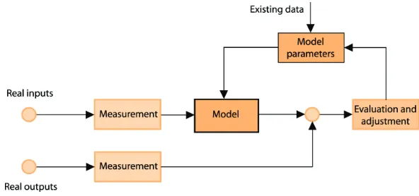
Modeling of hydrological phenomena in a basin includes complex interactions between the spatially distributed and closely related water flow processes, energy exchange and vegetation growth. All models try to describe these processes by a set of relatively simple mathematical expressions, the parameters of which have to be determined for each specific problem. Regardless of the model type, it is to a certain extent concentrated on a particular point in space and time. The consequence of this fact is that the majority of parameters cannot be determined by measurements, but they have to be evaluated by indirect methods. Calibration of model parameters is a process of determination of the parameter values with which the model produces lowest deviation relative to relevant observed values. In order to perform the calibration it is necessary to have the measured values of system inputs (rainfall, temperature etc.) and the respective system outputs (for example, the discharge on the outlet profile). As the dependence of the output upon model parameters is usually highly non-linear, direct regression methods cannot be applied and the calibration procedure has to be an iterative process. The model must meet certain requirements for the calibration to be feasible. Firstly, the interconnection between inputs, state variables and outputs must be consistent with measurements performed in the basin. Next, model results must be accurate and precise, i.e. they have to demonstrate minor value scattering and without unreliability of results. Finally, model structure and behavior must be in line with the applicable hydrological theory. The last condition is very important when the model should be used for testing of different scenarios regarding model state, for example, of the impact of various land uses on model behavior.
Fig. 1. Rainfall-runoff model calibration process
Since manual calibration is based on subjective estimations, an experienced hydrologist can perform very successful parameter estimation on the basis of his/her previous experience. However, the process can be time consuming and since it is based on expert evaluation, it requires time for training and acquisition of experience. Besides that, the experience of one expert is often difficult to transfer to other experts in a simple way. These limitations have raised an increased interest in automated calibration methods.
The goal of automatic calibration is the use of computers in the implementation of the last level of manual calibration. The first-level calibration is still performed manually because this is an expert-type problem that is not very demanding physically and which is performed only once in the initial calibration phase. Level two is usually neglected. Finally, last level is automated by the means of various algorithms that can be efficiently applied under the conditions of the high interdependency between the parameters and the nonlinearity of the model. Regardless of the selected algorithm, the issue of solution quality is an important one. The quality is defined by one or more mathematical expressions called the objective functions that are used for “navigation” of the calibration process to the optimum solution, i.e. the minimum deviation from the observed hydrograph (Prohaska et al., 2004).
The objective function is usually some form of error sum in the instance of time when the hydrographs are compared and the error is defined as the deviation of the calculated value from the observed one:
obs
t t
e
y y
(1)where e
is error, obs ty the value observed at time t, yt
the calculated value at time tand
a vector of the proposed model parameters.The most common objective function is the weighted sum of the squares of errors:
21 n
obs
t t t
t
F w y y
(2)where wt is the weight, or weighted coefficient at the time t, and n denotes the number of
points to be compared. If the values of all weights are equal to 1.0. the formula turns into the simple sum of square of errors.
2 1 2 1 1 n obs t t t n obs obs t t y y F y y
(3)wherein yobsis mean value of all observed data used for comparison with simulation results.
Nash-Sutcliffe coefficient can have values between -∞ and 1. Coefficient value of 1
corresponds to the perfect congruence between the model and the observed data. If the value of the coefficient is 0. that means that the model is equally efficient as the average value of the measured data. If the coefficient value is negative, the model is less efficient than the simple mean value. Therefore, the closer the coefficient is to 1, the closer the model is to the behavior of the real system.
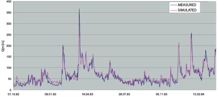
As an addition to the numerical evaluation of the congruence it is possible to perform a graphical comparison, which provides for the visual comparison of the correspondence between calculated and real elements of the hydrological system. An elementary comparison can be performed by the analysis of the comparative representation of the measured and simulated hydrographs.
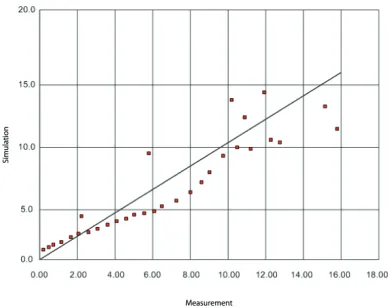
Fig. 2. Deviation of model parameters from the real values
Fig. 3. Presentation of errors in the calibrated model
The third method consists of the calculation and plotting of the time-series of errors – the differences between the calculated and real discharges. An example of this method is shown in Figure 3. Present diagram shows how the forecasting errors are distributed during the simulation time. The analysis of this diagram can help in identification of the parameters that may require additional attention in the calibration procedure.
Fig. 4. Comparative representation of measured and simulated values on a hydro-profile
4. Proposed calibration and validation procedure for the rainfall-runoff model based upon the SWAT algorithm
4.1. Basic principles of the proposed procedure
necessary to determine which parameters are to be calibrated and that should be performed in line with the quality of the applied data used and the performances of the algorithm itself.
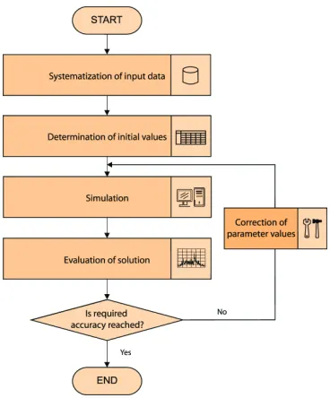
A systematic search of the best (optimum) parameter value is performed by the procedure shown in Figure 5. Calibration is performed in several steps, as follows:
Systematization of the required data,
Selection of calibration parameters, ranges of values and initial values,
Simulation,
Estimation and comparison of solutions and
Parameter correction and, eventually, a new simulation.
Fig. 5. Calibration algorithm
The first step of the procedure is the systematization of available data and an analysis according to the requirements already mentioned in the context of the selection of the calibration and validation period.
The next step is the determination the parameters to be estimated, of the range of their acceptable values and of their initial values. Same as in the case of any other search, the better the estimation of the initial values is, the faster should the desired solution be identified. Some of the initial parameter values and the ranges of their values can lie outside the expected boundaries, for the purpose of compensation for the initial data deficiencies.
The following three steps are iteratively repeated until the satisfactory solution is reached. The simulation is always performed with a new set of parameters. Simulation result is a hydrograph on a certain hydro-profile with the representative hydrological station and reliable measurements of discharge.
evaluation of model calibration quality that can be performed by many models and some of them will be presented below.
4.2. Selection of the parameters to be calibrated
The selection of the parameters to be calibrated is problem that must be solved in line with the indicators of input data quality (GIS data, hydro-meteorological data etc.). For example, if GIS data is of high quality, usually it is not necessary to significantly change the values of the parameters, such as CN (the parameter that reflects the land type and use). However, if the data is of a poor quality, or low accuracy, the deficiencies will have to be substituted for by the “artificial” parameter values. Also, due to the lack of accuracy in measurements of temperature and precipitation, and due to the fact that the major portions of time-series were filled up with a certain degree of reliability, it will be necessary to look for parameters concerning the snow pack formation and melting temperature in, seemingly, inappropriate ranges of values.
Bearing in mind the above, the model needs to be subjected to an additional analysis of its sensitivity to parameter changes. The change in model results is a reaction to a change in the value of a model parameter. The change in the result due to a unit change in the value of the certain parameter is defined as model sensitivity to parameter value change. Model sensitivity can be also presented as a derivative of model result over the observed parameter.
Sensitivity analysis of model parameters gave the main guidelines for the selection of the parameters to be estimated. Of course, there are several parameters that are, undoubtedly, very important for the results, and the sensitivity analysis has only confirmed their importance.
The groups of the most important parameters, as well as the most important parameters within the groups, have been selected on the basis of sensitivity analysis and the analysis of input data reliability.
The parameters for calculation of the referent input values are as follows:
plaps(mm/km) – rainfall gradient,
tlaps(oC/km) – gradient of temperature drop with an increase in altitude,
SW0(mm) – the initial state of soil humidity,
sno0(mm) – the initial value of water content in the snow pack,
Hwtbl0(m) – height of underground water layer,
Ts r (oC) – base temperature for the start of formation of the snow pack,
6
melt
b (mm/(day oC)) – snow melting factor for June, 21st,
12
melt
b (mm/(day oC)) – snow melting factor for December 21st,
Tmelt(oC) – snow melting base (referent) temperature (close or equal to zero),
snocov(%) – percentage of snow coverage on the hydrological unit,
sno100(mm) – the minimum snow height measure for snow coverage of 100%,
canday(mm) – the maximum water volume to remain on plants in a given day,
canmax(mm) – the maximum water volume to remain on fully grown plants,
LAI(%) – total area of green leaves per surface area in a given day,
n(m-1/3s) – Manning coefficient for the particular vegetation type,
b(kg/m
3) – soil specific weight,
mc(%) – percentage of clay content in the soil,
AWC (mm) – required water capacity of soil as a function of the vegetation blanket
that represents the necessary amount of water in the soil, required for the normal growth and development of the particular vegetation cover,
SAT (mm) – water content in the completely saturated soil,
surlag (-) – lag coefficient of the surface runoff,
k and x (-) – parameters defining the open-channel flow in the sub-catchment within a
complex basin,
ksurf (%) – weighting factor for the surface runoff distribution and
kgw (%) – weight for the subsurface runoff distribution.
For each of the calibrated parameters, the interval of the possible values, as well as the initial values for the calibration must be defined.
The parameters to be calibrated can be divided into the four groups: the parameters related to vegetation, the parameters related to pedology, the parameters related to hydrogeology and other parameters (that describe data correction, snow pack formation and snowmelt and flow in open channels).
Parameters related to vegetation
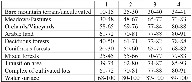
One of the most important parameters is the CN (Curve Number) parameter, defined as the
family of curves, specific value of which is related to the combination of dominant vegetation on a hydrological unit and the dominant pedology class.
1 2 3 4
Bare mountain terrain/uncultivated 10-15 25-30 30-40 34-41
Meadows/Pastures 30-48 48-67 65-77 73-83
Orchards/Vineyards 58-65 69-76 77-84 80-88
Arable land 61-72 70-81 77-88 80-91
Deciduous forests 40-50 61-71 72-82 78-88
Coniferous forests 20-30 50-60 65-75 68-82
Mixed forests 25-45 55-66 70-77 77-83
Transition area 39-74 62-80 74-87 85-93
Complex of cultivated lots 61-72 70-81 77-88 80-91
Water surface 68-100 80-100 87-100 89-100
Table 1 shows the ranges of possible values of this parameter.
Parameters related to pedology
The most important parameter to be calibrated that is, directly related to the soil type or soil class, is Ksat.
CLASS Ksat (mm/h)
Mould/dark soil 2 11-110
Brown forest soil 3 1.1-11
Podzolic and parapodzolic soil 2 11-110
Recent alluvial sediments 1 110-400
Rendzina on solid limestone 3 1.1-11
Gravel and conglomerate 1 110-400
Grey soil on limestone 2 11-110
Grey soil on slate 2 11-110
Clay soil 4 0.001-1.1
Table 2. Ranges of the possible values of the soil parameter Ksat
Table 2 represents the ranges of the values of this parameter for one soil class.
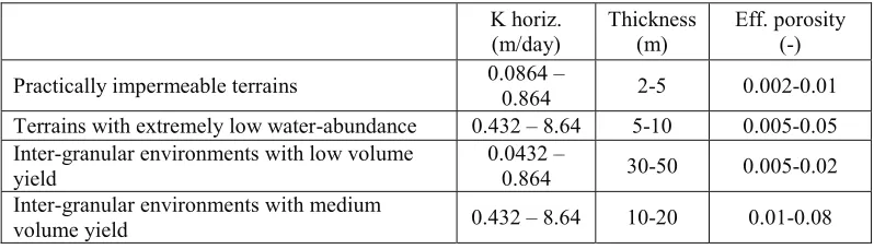
Parameters related to hydrogeology
Parameters related to hydrogeology to be calibrated are shown in Table 3. The most important
parameter is the lag coefficient of the subsurface runoff gwlag.
K horiz.
(m/day) Thickness (m) Eff. porosity (-)
Practically impermeable terrains 0.0864 – 0.864 2-5 0.002-0.01
Terrains with extremely low water-abundance 0.432 – 8.64 5-10 0.005-0.05
Inter-granular environments with low volume
yield 0.0432 – 0.864 30-50 0.005-0.02
Inter-granular environments with medium
volume yield 0.432 – 8.64 10-20 0.01-0.08
Table 3. Ranges of the possible values of hydrogeological parameters
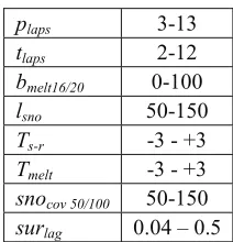
Other parameters
This group includes the parameters related to the correction of precipitation and temperature
relative to the change in elevation above the sea level plaps, tlaps, then the parameters related to
snow storage and melting bmelt6, bmelt12, lsno, tsr, tmelt, snocov100.snocov50. as well as the parameter of
surface runoff lag, surlag, initial soil humidity, SW0. initial height of the water table, hwtbl0 and
plaps 3-13
tlaps 2-12
bmelt16/20 0-100
lsno 50-150
Ts-r -3 - +3
Tmelt -3 - +3
snocov 50/100 50-150
surlag 0.04 – 0.5
Table 4. Approximate ranges of possible values of other model parameters
4.3. Base values for parameter calibration
Before the start of the iterative procedure of calibration it is necessary to determine the initial values of the selected parameters. The success in the selection of an initial value can have a substantial impact on the duration of the calibration. The closer are the initial values to the optimum parameter values, the faster will the calibration process go.
Parameters related to vegetation
The initial values of the CN parameter, based upon the ranges shown in Table 1, are the result
of the process of parameter calibration, performed on the selected River Drina basin and they are shown in Table 5.
1 2 3 4
Bare mountain terrain/uncultivated 12 27 35 39
Meadows/Pastures 35 55 70 77
Orchards/Vineyards 60 72 80 84
Arable land 65 75 82 85
Deciduous forests 45 65 77 82
Coniferous forests 25 55 70 70
Mixed forests 30 60 73 80
Transition areas 50 70 80 90
Complex of cultivated lots 65 75 80 85
Water surfaces 80 90 90 95
Table 5. Initial (calibrated) values of the CN parameter depending on vegetation type and soil class
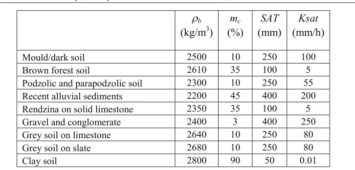
Parameters related to pedology
The initial values of the parameters b, mc, SAT and Ksat have been determined according to the
physical characteristics of the soil (the first three) and they are the result of the process of
b(kg/m
3)
m
c(%)
SAT
(mm)
Ksat
(mm/h)
Mould/dark soil 2500 10 250 100
Brown forest soil 2610 35 100 5
Podzolic and parapodzolic soil 2300 10 250 55
Recent alluvial sediments 2200 45 400 200
Rendzina on solid limestone 2350 35 100 5
Gravel and conglomerate 2400 3 400 250
Grey soil on limestone 2640 10 250 80
Grey soil on slate 2680 10 250 80
Clay soil 2800 90 50 0.01
Table 6. Initial (calibrated) values of the parameters depending on the soil type
Parameters related to hydrogeology
The initial values of the parameters of hydrogeological classes, based upon the ranges shown in Table 3, are the result of the process of parameter calibration performed on the selected River Drina basin – Table 7.
K horiz.
(m/day) Thickness (m) Eff. porosity (-)
Practically impermeable terrains 0.01 3 0.01
Terrains with extremely low water-abundance 2,3 8 0.05
Inter-granular environment with a low volume yield 0.4 40 0.02
Inter-granular environment with a medium volume yield 4,2 15 0.08
Table 7. Initial (calibrated) values of the parameter of hydrogeological classes
Parameters related to the sub-catchment
The initial values of the parameters related to the sub-catchment, based upon the ranges shown in Table 4, are the result of the process of parameter calibration performed on the selected River Drina basin – Table 8.
plaps 4
tlaps 5
bmelt16/20 55 lsno 0.5
Tstor 1
Tmelt 0
snocov 50/100 80 surlag 0.2
4.4. Selection of the Calibration and Validation Period
Calibration, as mentioned above, is a process of model testing with known input and output values, aimed at the adjustment or evaluation of certain parameters. In contrast to calibration, validation is the comparison of model results with an independent data set (without further adjustment). This is the way to confirm the correctness of the calibrated model.
Conditions to be met by these two periods are as follows:
The two periods must be different that is, they have to be two separate and independent
time periods,
Both intervals must have a similar range of rainfall and runoff,
Selected time periods must be appropriate for simulation of all possible conditions and
Impact of inaccuracy of filling missing input data must be mitigated.
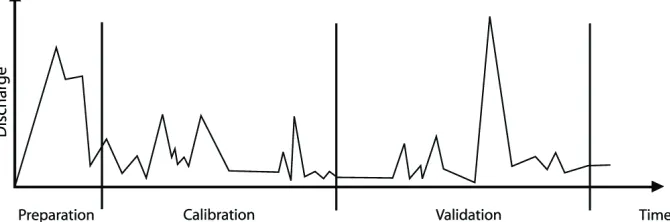
Fig. 6. Selection of the parameter calibration and validation period
In order to verify the model during the period which was not used for its calibration, the calibration period and the validation period must be two separate and independent time periods. This is the way to come to realistic conclusions on model’s response under the conditions not covered by the calibration. Selected periods have to include as many phenomena as possible, such as heavy and intensive rainfall, dry seasons, extreme and medium winters etc. Should some of these phenomena be neglected, then it might happen that the parameters related to the given conditions might be under- or over-estimated.
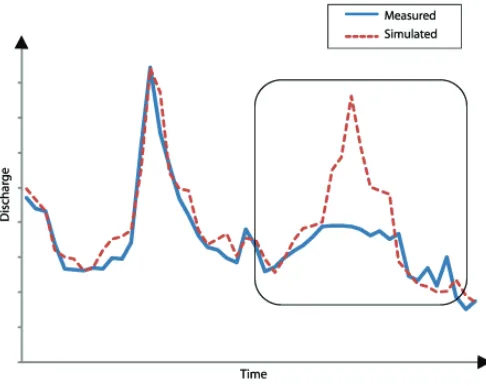
It is extremely important to pay attention to the importance of the relative accuracy in filling-in of the time-series for rainfall, temperature and discharge. A bad impact that the filled-in data can have on model behavior is illustrated filled-in Figure 7.
Figure 7 shows a hypothetical case of an calibrated model, with small number of errors relative to the measured data in 80% of the validation period. However, it generates the outstanding runoffs in the short period, even though the base runoff is dominant in the measured data.
Fig. 7. Impact of filled-in series on parameter calibration
4.5. Selection of the optimization algorithm
The pronounced high nonlinearity and numerous parameters make the identification of the optimum parameter set difficult, because it is not possible to forecast model behavior in all cases of their change. The problem of calibration in this type of models may be treated as a complex optimization problem. As the calibration is performed for a long time interval, the cause and the occurrence of a certain phenomenon is often difficult to forecast, because they are dependent upon numerous other parameters of the system. This may be interpreted as a mixed problem that is based upon the generation and evaluation of numerous solutions that require observance of a broad set of equations and inequalities, as well as logical limitations. Solving this type of problem by classical methods (gradient methods, dynamic programming methods, scenario selection methods etc.) is very difficult. That is the reason why the use of parallel genetic algorithms is proposed. The selection of evaluation methods provides extendibility and ability to adapt and improve without violation of the basic algorithm.
Genetic algorithms (GA) were proposed by John H. Holland in early 70's of the last century (Holland, 1975). For more than two decades and particularly in the last several years, they proved to be very powerful and able to serve as a general tool for solving a series of problems arising from the engineering practice. This can be explained by their simplicity – the simplicity of the idea they are based on itself, of their application, as well as by the contribution made by many scientists and engineers who worked on their adaptation to many problems and the improvement in their efficiency. Simultaneously with the expansion of their application, the research related to the operation and features of the genetic algorithms has also expanded, and efforts are made to reduce their elements to theoretical foundations. Unfortunately, the results of the theoretical research are not unambiguous and genetic algorithms remain to this day basically heuristic methods (Goldberg, 1989).
Evolution strategies, which were developed in Germany in the 60's of the last century, share many common features with genetic algorithms and very often it is difficult to determine the boundaries between them when different variants of both approaches are considered. Both methods operate on a population of solutions upon which defined operations are iteratively applied. That is why the phases of such a process are called generations, after the model of natural evolution.
The strength of genetic algorithms comes from the fact that they can determine the position of the global optimum in the space with multiple local extremes, i.e. in the so-called multimodal space. The classic deterministic methods are always heading towards a local minimum or maximum, which can be also global, but this cannot be determined from the results. Stochastic methods, and, consequently, genetic algorithms, are not dependent upon the initial solution and they can be used to locate the global optimum of an objective function with a certain probability by its search procedure.
The main difference in application between the classical and stochastic methods lies in the fact that for the results of the, for example, gradient method, one can safely claim that a local extreme has been reached with a desired accuracy. However, in the case of application of genetic algorithms one cannot claim with absolute reliability that the obtained result represents a global or just a local optimum, and whether it has been determined with the desired accuracy. No matter how much the performance of stochastic methods should be improved, they will never yield results with absolute reliability. The reliability of results is significantly improved with the repetitions of the solution process, which does not make sense for classic methods. Ever since the genetic algorithms have been invented, great attention was paid to research aimed at the improvement of their efficiency.
5. Calibration of SWAT based model by parallel genetic algorithms
5.1. Parallel genetic algorithms in general
Parallel genetic algorithms are used for the solution of difficult optimization problems. Difficult problems require big populations and long chromosomes, what leads to the long duration of the process. The main reason for the parallelization of genetic algorithms is a need for the acceleration of their execution on multiprocessor computers or several computers operating in a network. In the early days of development of genetic algorithms, the attempts were made to assess parallelization impact on algorithm performance, such as the speed of convergence. Namely, beside the speed, some models of parallel GAs have showed better performance in comparison to the same sequential (serial) algorithm: they are able to yield better solutions with less iteration than the corresponding sequential GA (Cantú-Paz, 1995). However, this is a special case when the parameters of the sequential GA are not set well. In reality, the goal is to have PGA with the same features as the corresponding sequential GA with well set parameters.
In the first case, only the process of evaluation is parallelized. Same as for the sequential genetic algorithm, the operators act on just one, common, population. This type of model is called the single-population model. In the second case, the population is divided into several subpopulations; hence, such a model is called the multi-population model, i.e. the GA is called the multi-population parallel genetic algorithm (Cantú-Paz 1998, 1999; Talbi 1991). A reduction of the multi-population PGA execution time is to be expected, because the subpopulations contain fewer individuals than the initial populations in the single-population model.
There are several possible levels of GA parallelization: at the level of a population, at the level of an individual and at the level of the evaluation. According to the level of parallelization, there are three basic ways to divide a sequential GA into subtasks: coarse-grained GA, fine-grained GA and master-slave GA.
A coarse-grained division is the division of big populations into smaller parts – subpopulations. In this case a decomposition approach, or the above mentioned multi-population parallel GA is present, and it is decomposed in such a manner that several GAs can be executed in parallel on smaller populations.
A fine-grained division is an extreme form of division of a big population into subpopulations with a size of one individual. Each processor executes the genetic operators on individuals assigned to it and the neighboring individuals. This division is also a representative of a multi-population model.
It is also possible to perform in parallel an evaluation while genetic operators are executed sequentially. This division is called “master” and “slave”. The master performs GA on the common population; hence that is a single-population model. In each iteration the slaves perform a parallel computation of the objective function values, after the master has performed its sequential part of the work.
5.2. Application of parallel genetic algorithms in calibration of the SWAT-based models
As several approaches to GA parallelization are applicable, it is important to note that only the master-slave model and the similar global parallel GA have the same features as the sequential GA; hence, all theoretical considerations of sequential GA are applicable to them, as well. The other models significantly change the way the execution of the algorithm, thus, the theoretical analysis of the operation of those algorithms is still in a development stage (Cantú-Paz, 1995).
One of the criteria for the selection of GA parallelization method is the hardware the algorithm is to be executed on. Considering the fact that the computers are LAN networked (one of the commonly available resources for parallelization), a logical choice would be the master-slave model. In order to implement a parallel GA, it would be necessary to define several steps: presentation (coding) of the solutions, determination of fitness (calculation of the objective function), crossover, mutation and selection. All steps are analyzed in detail below.
Presentation of the solution
boundaries for each individual parameter. If min
i
P and max
i
P denote the minimum and maximum
values of parameter i, than the number of segments is defined as
max min i i P P n
(4)
where is the required accuracy, while n is the total number of segments within the interval.
In order to perform a simulation based on a binary-coded solution, the specific values of
each parameter should be determined in the decimal form. If
1,n is the integer value of thesegment for the parameter i, than its specific value,Pi, which is used for setting of the
SWAT-based model before simulation, can be defined as
max minmin 1 i i
i i
P P
P P
n
(5)
Determination of solution fitness
The determination of solution fitness is directly related to the nature of the optimization problem. Therefore, for the purpose of model calibration it is necessary to define the normalized error index. Its integral evaluation is based on the square root of the sum of squared errors, weighted by observed peaks, which represents the balanced implicit measure of the comparison of the intensity of peaks, volumes and times of occurrence of peaks of the two hydrographs, where neither base nor surface runoffs are favored. This function compares all ordinates by squaring the differences and weighting the squared differences. Weighting coefficient assigned to each ordinate is proportional to the value of the ordinate. Ordinates with values higher than the mean value of the observed hydrograph are assigned with weighting coefficients higher than 1, and those with lower are assigned with coefficients less than 1. Ordinate of the observed maximum (peak) is assigned with the maximum value of the weighting coefficient. Then, the sum of these weighted squares of differences is divided by the number of ordinates of the computed hydrograph; the aim of this procedure is to identify the mean squared error. The calculation of the square root of that value leads to the square root of the mean squared error:
( )
1 ( ( ) ( ))2
2 1
NQ Q i Q
M M
J QM i Q iS
NQ i QM
(6) where :
J – error norm,
NQ– number of calculated hydrograph ordinates,
Q i
M( )
- real discharge, Q iS( )- calculated discharge, determined upon the selected set of model
parameters and
QM - mean value of the real discharge.
Crossover
In the process of crossing participate the two individuals – “parents”, and crossing generates one or two new individuals – “offspring”. The most important characteristic of crossover is that the offspring inherits the characteristics of the parents. If the parents are good (i.e. if they have passed the selection process) most probably the offspring will be of good quality too, if not better than the parents.
It is assumed that exactly this crossover operator is what makes the genetic algorithm different from other optimization methods. This does not apply to the mutation operator which is also found in simulated annealing and evolutionary strategies. In the subject case of calibration, the crossover in a single point is applied.
Mutation
After the recombination, offspring passes through the mutation process. Offspring variables are varied for small random values (mutation step), with low probability. The probability of variable mutation is in inverse proportion to the dimension of the individual (the number of variables). The more variables are contained in an individual, the lower is the mutation probability. The mutation searches through the solution space, and the mutation itself is the mechanism used in order to avoid local minima. Namely, if the entire population ends up in a local minimum, the only way to find a better solution is to perform a random search through the space of acceptable solutions. It suffices to find a single individual (created by mutation) which is better than the other ones, to have all the individuals moved to the space with better solutions during the next several generations. The role of the mutation is also to renew the lost genetic material.
Selection
The purpose of selection is the preservation and transfer of good characteristics upon the next generation of members. The selection is used for the choice of the good individuals that will participate in the next step – the reproduction. This is the way to preserve and transfer the good genes or the good genetic material upon the next population, while the bad ones disappear. Selection procedure could be performed by simple sorting and selection of the best individuals. However, such a procedure leads to a premature convergence of the genetic algorithm, i.e. the optimization process is practically finished in just a few initial iterations. The problem encountered here is the fact that this procedure leads to the loss of good genetic material that is possibly contained in the bad individuals. For that reason it is necessary to ensure that even the bad individuals have a certain (low) probability of survival. On the other hand, the good members should have a higher probability of survival, i.e. they should have a higher probability in the reproduction process. The roulette wheel selection was used in the present example. This type of selection resembles the eponymous game of chance, since the selection of an individual is based on a random number (as when the roulette ball falls into one of the 36 holes by chance). The only difference as compared to the real game is that the size of the “hole” is proportional to the fitness of the individual that is, the individual with a better fitness has a greater chance to be selected.
5.3. Utilization of PGA for calibration of a SWAT model in the HIS application library
genes. The input files prepared in this manner are then forwarded to the individual workstations on the network, where the simulation and determination of fitness of each individual solution are performed. Crossover, mutation and selection take place on the server after the evaluation of all population individuals. The result of these operations is a new population which is again divided to the workstations for evaluation.
The Alchemi. NET platform was used for the implementation of the algorithm for estimation of model parameters according to the master-slave approach. The Alchemi platform is a library based on the .NET platform. It provides the infrastructure necessary for software solution development and implementation of software solutions in a distributed environment, the so-called “grid” (Setiawan et al., 2004; Nadiminti et al., 2004; Luther et al., 2005). The basic structure of the platform is shown in Figure 9. The main elements of the system are the manager, the users and the agents. The manager is the computer serving as the server for agent management on the basis of the assignments delivered by the system users. The manager has an updated list of active agents and their states and it performs their engagement, as well as the collection of the feedback messages and data. The communication infrastructure itself can be created in the range of connections within the dedicated network up to a combination of computers with Internet connections no matter how remote they may be.
Fig. 8. Parallelization scheme for GA calibration of SWAT model
The architecture of parallel system relies on the presence of dedicated high-performance computers in the local network. This is the way to establish an extremely fast communication (usually the bottleneck of all parallel systems) and avoid operational bugs that could occur should the network be accessed from the surrounding environment. On the other hand, grid architecture relies on a large number of individual computers connected to a slower network, which are not intended only for the grid operation. Of course, if a separate isolated network with good performances is used and the computers are optimized for the operation in the grid the better results can be achieved. The actual network used for the estimation of model parameters presented in this paper comprised of over 20 worker agents, with various hardware configuration.
6. Presentation of the model to be calibrated
An example of estimation of the parameters of the SWAT model is presented below. The selected example represents the basin of the selected river up to the dam with storage, where parameters are evaluated according to the observed discharges (before the dam was constructed).
Fig. 10. The River Drina basin between the hydro-profiles “Bajina Bašta” and “Višegrad”
The total area of the basin that encompasses the “Bajina Bašta” storage is 14232 km2, or
73.98 % of the River Drina basin. Simulation period is from September 1st, 1997 to September
1st, 1999. Hydro-profile “Višegrad” is shown as the source with the assigned discharge, which
discharges on the hydro-profile “Bajina Bašta” (dam). The resulting hydrograph is the result of the calculation using the SWAT-based rainfall-runoff model.
7. Results
Below are shown the results of calibration of model parameter according to a predefined criterion for the whole River Drina basin (Figure 11) and, particularly, the result of the chosen example of parameter estimation using the SWAT-based model presented in Chapter 6.
7.1. “Bajina Bašta” – dam
Comparative illustration of measured and simulated values shows satisfactory correspondence between the observed and simulated hydrographs (error estimation according to the predefined criterion (6) is 3.111). This was to be expected, as the impact of the rainfall-runoff model is decreasing due to the operation of the upstream object “Višegrad” and several apparent deviations are the result either of the fact that the parameters were taken from other basins or of the unreliability of measured data.
Fig. 13. Deviations of simulation results on hydro-profile “Bajina Bašta” – dam from the real values
Diagram of deviations of model parameters from the real values shows that the grouping around the middle line is satisfactory and that there are not many major deviations (except for a certain percentage of points), with a weak tendency towards a deficiency of the simulated inflows relative to historical data.
The error diagram for the calibrated model in time shows a balanced error distribution during the entire period, i.e. it shows that the balance has been reached, but that the peak values were translated in time by one or two steps.
Fig. 14. Model error on hydro-profile “Bajina Bašta” in time
One can conclude that the quality of the basin calibration upstream from the hydro-profile “Bajina Bašta” is satisfactory, both in terms of balance and discharge dynamics.
7.2. The River Drina Basin – whole basin
8. Conclusions
Automatic calibration of the rainfall-runoff hydrological model is more and more often based on the use of genetic algorithms. This trend is not surprising, being that the number of parameters for these models, as well as the search space, is huge. However, sequential GA are in these cases often time-consuming, so the calibration may last for several days, weeks, or even months. In order to make the duration of the calibration process acceptable, it is necessary to divide major sequential problems into the sub-problems and to parallelize their solutions. This paper presents the platform for the calibration of a SWAT-based model, founded on parallel GA, implemented on a LAN of computers, which is changeable both in structure and the number of computers taking part in the calibration process. Additionally, the paper presents the procedure of preparation of calibration data, as well as the procedure of selection of calibration and validation periods.
Further researches will be focused on the introduction of additional mechanisms for parallel GA improvement, such as the adaptive parameters of mutation, selection and crossover. This is the way to strive for a better solution convergence, resulting in additional acceleration of the calibration process.
References
Arnold JG and Allen PM (1996), Estimating hydrologic budgets for three Illinois watersheds. J.
Hydrol. 176(1‐4): 57‐77.
Arnold JG, Srinivasan R, Ramanarayanan TS, Luzio MDi (1999), Water resources of the Texas gulf basin. Water Sci. Tech. 39(3): 121 - 133.
ASCE (1993), Criteria for evaluation of watershed models. J. Irrigation Drainage Eng. 119(3): 429-442.
Bracmort KS, Arabi M, Frankenberger JR, Engel BA, Arnold JG (2006), Modeling long-term water quality impact of structural BMPS. Trans. ASAE 49(2): 367-384.
Cantú-Paz E (1995), A Summary of Research on Parallel Genetic Algorithms.IlleGAL Report Number 95007, University of Illinois at Urbana-Champaign.
Cantú-Paz E (1998), A survey of parallel genetic algorithms. Calculateurs Paralleles, Reseaux et Systems Repartis. Vol. 10. No. 2. pp. 141-171. Paris: Hermes. ps.gz Abstract
Cantú-Paz E (1999). Topologies, Migration Rates, and Multi-Population Parallel Genetic Algorithms. GECCO 1999: 91-98
CEAP-WAS (2005), Conservation effects assessment project: Watershed assessment studies. Available at: ftp://ftp-fc.sc.egov.usda.gov/NHQ/nri/ceap/ceapwaswebrev121004.pdf. Accessed 15 August 2005.
Goldberg DE (1989), Genetic Algorithms in Search, Optimization, and Machine Learning.
Reading, Mass.: Addison‐Wesley, 1989.
Holland JH (1975), Adaptation in Natural and Artificial Systems. Ann Arbor, Mich.: University
of Michigan Press.
Legates DR and McCabe GJ (1999), Evaluating the use of “goodness-of-fit” measures in hydrologic and hydroclimatic model validation. Water Resources Res. 35(1): 233-241. Luther A, Buyya R, Ranjan R, Venugopal S (2005), Alchemi: A .NET-Based Enterprise Grid
Computing System, Proceedings of the 6th International Conference on Internet Computing (ICOMP'05), June 27-30, 2005, Las Vegas, USA.
Parker R, Arnold JG, Barrett M, Burns L, Carrubba L, Crawford C, Neitsch SL, Snyder NJ, Srinivasan R, Williams WM (2006), Evaluation of three watershed-scale pesticide fate and transport models. J. American Water Resources Assoc
Prohaska S, Simic Z, Milivojevic N, Orlic A, Ristic V (2004), Rainfallrunoff modelling based on the SWAT model, XXII Conference of the Danubian countries on the Hydrological forecasting and Hydrological bases of water management, Brno, 2004.
Refsgaard JC (1997). Parametrisation, calibration and validation of distributed hydrological models. Journal of Hydrology, 198, 69-97.
Simić Z, Milivojević N, Prodanović D, Milivojević V, Perović N (2009), SWAT-Based Runoff
Modeling in Complex Catchment Areas – Theoretical Background and Numerical
Procedures. Journal of the Serbian Society for Computational Mechanics, Vol. 3, No. 1
Saleh A J, Arnold G, Gassman P W, Hauk LM, Rosenthal WD, Williams JR, MacFarland AMS (2000). Application of SWAT for the upper North Bosque River watershed. Trans. ASAE 43(5): 1077-1087.
Santhi C, Arnold JG, Williams JR, Dugas WA, Srinivasan R, Hauck LM (2001). Validation of the SWAT model on a large river basin with point and nonpoint sources. J. American Water Resources Assoc. 37(5): 1169-1188.
Santhi C, Srinivasan R, Arnold JG, Williams JR (2006). A modeling approach to evaluate the impacts of water quality management plans implemented in a watershed in Texas. Environ.
Model. Soft. 21(8): 1141‐1157.
Setiawan A, Adiutama D, Liman J, Luther A, Buyya R (2004), GridCrypt: High Performance Symmetric Key using Enterprise Grids, Proceedings of the 5th International Conference on Parallel and Distributed Computing, Applications and Technologies (PDCAT 2004, December 8-10, 2004, Singapore), Springer Verlag Publications (LNCS Series), Berlin, Germany.
Singh J, Knapp HV, Demissie M (2004). Hydrologic modeling of the Iroquois River watershed using HSPF and SWAT. ISWS CR 2004-08. Champaign, Ill.: Illinois State Water Survey. Available at: www.sws.uiuc.edu/pubdoc/CR/ISWSCR2004-08.pdf. Accessed 8 September 2005.
Talbi E-G, Bessiere P (1991). A Parallel Genetic Algorithm for the Graph Partitioning Problem. In Proc. of the International Conference on Supercomputing, Cologne, June 1991.
Van Liew MW, Veith TL, Bosch DD, Arnold JG (2007). Suitability of SWAT for the
Conservation Effects Assessment Project: A comparison on USDA‐ARS watersheds. J.
Hydrol. Eng. 12(2): 173‐189.
Wang X and Melesse AM (2005), Evaluation of the SWAT model’s snowmelt hydrology in a northwestern Minnesota watershed. Trans. ASAE 48(4): 1359-1376.