PARALLELIZATION, SPATIAL DECOMPOSITION AND LOAD
BALANCING OF A SINGLE TREE LEVEL FOREST DYNAMICS
SIMULATOR
Artur Signell
1, Johan Sch¨
oring
2, Mats Aspn¨
as
3, Jan Westerholm
41Ph.D. Student,2Res. Assist.,3Lecturer,4Professor. ˚Abo Akademi University, Joukahainengatan 3-5, 20540 ˚Abo, Finland
Abstract.SPATE-HPC is a single tree level forest dynamics simulator capable of simulating very large
forest areas. The size and shape of the simulation area as well as the number of trees are only restricted by the amount of memory available and subareas can be used for a tighter specification of the simulation. In this article we describe the parallelization of SPATE-HPC and its major computational challenges. We describe the domain decomposition methods and the load balancing strategy we have used to ensure good performance and scalability of huge simulations. We also describe how we have verified the correctness of the parallel implementation. Additionally we present performance measurement results for the simulator by running a fixed 32,300 ha simulation on 32-2,048 processors and a simulation with 1,000 ha/core on 32-2,048 cores. The results show that it is possible to simulate a forest area of more than 1,000,000 ha with several billion trees.
Keywords: Forest dynamics simulation, individual tree, high-performance computing, parallel pro-gramming
1
Introduction
The forest industry and individual forest owners are very interested in creating well functioning and produc-tive forests by using various silvicultural methods and thinning practices. Experimental studies of these meth-ods are tedious to perform, particularly due to the long time perspective involved, and therefore forest dynamics simulators have been developed. Forest dynamics simu-lators can be classified based on the modelling unit used (Porte and Bartelink 2002): whole stand and single tree. Whole stand simulators are based on stand level mod-els usually with no individual tree information. Single tree simulators are based on a tree model and a list of trees. A simulated tree can be a representation of one or several real trees. Single tree level simulators can fur-ther be classified into dependent and distance-independent based on if intertree distance information is used in the simulation or not. Gap simulators, which are a kind of single tree simulators but simulate only small forest patches, are sometimes included as a sepa-rate class.
Several implementations of the different simulator types exist, all with their own capabilities and limi-tations. Stand level simulators are typically
compu-tationally very efficient but produce coarser level out-put, whereas single tree simulators, especially distance-dependent, are computationally more heavy but can per-form more fine-grained operations and produce more de-tailed output. In many single tree level simulators (e.g., Harja and Vincent (2008), Pretzsch et al. (2002), Col-igny et al. (2003)) the simulation area is limited in size, to a few hectares, or in shape, to a rectangle or square. There might also be a limitation regarding number of trees.
SPATE-HPC is a distance-dependent single tree level forest dynamics simulator which imposes very few re-strictions on the simulation. The simulation area can be of any size and shape which makes it possible to simulate real forest areas in addition to hypothetical ones. The simulation area can also be divided into sub-polygons to take into account different conditions in different parts of the forest. SPATE-HPC is designed to be able to sim-ulate anything from small forest stands to huge forests on a landscape scale. The number of trees is restricted only by the amount of computer memory and each tree in the simulation is directly mapped to a real tree so in-dividual trees’ properties can be taken into account e.g. when making thinning decisions.
In this article we describe the parallelization of
Copyright c2010 Publisher of the International Journal ofMathematical and Computational Forestry & Natural-Resource Sciences
Figure 1: Sample area of 35 hectares from a digital map of Nurmes, Finland.
SPATE-HPC and the challenges encountered in making the simulator able to efficiently simulate areas up to and above 1,000,000 ha containing more than 1,000,000,000 trees. In section 2 we briefly present the simulator and the models used in simulation. In section 3 we describe the issue with locating tree competitors and how it has been solved in the simulator. In section 4 we describe how the simulator has been parallelized, the domain de-composition method used and the communication be-tween processes. Section 5 describes the load balancing issues faced and how they have been solved, and in sec-tion 6 we briefly describe what we have done to ensure that the parallel version has been correctly implemented. We conclude by providing scalability and performance results of the simulator in section 7.
2
SPATE-HPC
SPATE-HPC is a single tree level, time step based simulator which simulates tree growth, mortality, repro-duction and forest management. The length of the time step is user definable and typically chosen to be 1-10 years. The simulation area is unrestricted in size and shape and can be divided into several compartments. A compartment is a polygon-shaped area with global pa-rameters for the area and for the trees inside it. An example of a compartmentalized simulation area can be seen in Figure 1.
The simulator uses a distance dependent competition model where trees close to each other compete while trees farther away than a certain distance, the compe-tition distance, do not affect each other directly. The competition area for a tree is defined as a circle with the competition distance as radius, centered on the tree. The competition is based on distance only and is not restricted by compartment borders. A more complex competition area than a circle, e.g. a polygon, could be
used as long as there is an efficient method to detect if a point (another tree) is inside the competition area.
The model presently implemented in SPATE-HPC is a linear stochastic simulation model (Lin 2003), which has the form expressed by eq. 1, however the simulator can be modified to use any model where interactions between trees are local.
Y =xβ+ (1)
This model is used to calculate a propertyY (e.g. di-mension or height) for a target tree. Both xandβ are vectors containing one or more elements. Each element in x consists of a competition index for the tree or a combination of competition indices for the tree. The competition indices are dependent on the tree or its sur-roundings (e.g. tree diameter, average distance or tree density inside the competition area). The elements inβ are calculated using the linear model in eq. 2 to allow each βi to depend on the target tree.
β =a∗1β1∗+a∗2β2∗+. . . (2) In eq. 2 each a∗i is a factor related to the current tree. Possible values are for instance tree age, diameter or a tree species coefficient. The β∗ values are parame-ters specified by the user to weigh the a∗i factors. The variablein eq. 1 is a pure random component.
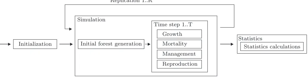
2.1 Simulation flow The program flow, as shown in Figure 2, consists of initialization, simulation and statis-tics output. First the simulator is initialized based on given input parameters (simulation area, model parame-ters etc). Then the actual simulation is performed, con-sisting in turn of two main parts: initial forest genera-tion and time steps. In the initial forest generagenera-tion part the starting point for the simulation is set up while the actual simulation is done in the time steps. These are described in more detail below. Finally statistics (age structure, volume, removal, etc.) for each compartment and time step in the simulation are summarized and out-put.
For accurate statistical results it might be necessary to use multiple replications, i.e. run the simulation mul-tiple times using different random numbers. For each replication the initial forest generation and all time steps are simulated and aggregated data such as basal areas and volumes are stored. At the end of the replications average values for all the aggregated data are calculated.
Figure 2: Program flow
The user can provide input data on different levels rang-ing from only the number of trees within a compart-ment to the exact locations and properties of all trees in a compartment. If locations and/or properties are not provided by the user they are generated by the simula-tor. Tree locations are generated using a homogeneous Poisson process. When all trees have been placed the tree properties are calculated using the linear formula in eq. 1 using user defined parameters. Distributions for one or more properties can additionally be specified and these will be used to transform the generated properties to the given distributions.
2.1.2 Time steps In the time steps part the actual tree time evolution simulation is performed. Starting from the initial forest we simulate one time step at a time until the requested number of years has been simulated. Each time step is divided into 4 phases, executed in this particular order: growth, mortality, management and reproduction. All calculations in a time step are based on the state of the forest at the beginning of the time step, i.e. changes are not applied until at the end of the time step.
In the growth phase the growth for each tree is calcu-lated using eq. 1 by taking the individual tree’s competi-tion into account. The mortality phase determines which trees will survive the time step using regular (growth less than a given threshold) and irregular (using a lo-gistic model) mortality. Management is the only part of the program where external interaction with the for-est is simulated. The methods used for management are based on single tree properties which enables the usage of detailed management methods. In the reproduction phase the number of new seedlings to be generated is determined based on input parameters and the current compartment state. The new seedlings are placed into the compartments using a homogeneous Poisson process and their properties are calculated using eq. 1 and given parameters. For reproduction it is also possible to spec-ify a transformation of the properties like for the initial
forest.
3
Finding neighboring trees
There are two main types of operations in the simu-lator: those that operate on a compartment at a time (management, reproduction) and those that operate on all trees in the simulation (growth, mortality). For com-partment level operations it is essential that each tree is assigned to only one compartment so no compartment overlaps another compartment. Both types of operations operate on one tree at a time and take trees inside the tree’s competition area into account. For the operations to be efficient it is important to be able to quickly locate all trees inside a tree’s competition area.
The competition for a tree, consisting of the trees in-side the tree’s competition area, is not restricted by com-partment boundaries; all trees inside the competition area are included regardless of which compartment they belong to. To be able to locate competitors efficiently we utilize the cell-space partitioning technique (Buck-land 2004), which is a simple spatial indexing method based on a regular tessellation of the simulation area.
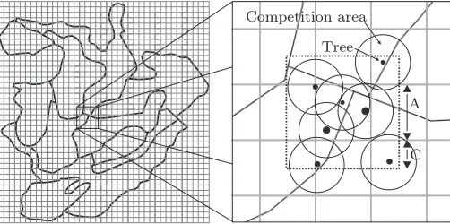
We set up the spatial index by overlaying the simula-tion area by a regular grid of cells, unrelated to compart-ment borders, as shown in Figure 3. Two mappings are set up for the cells. The first one links each tree to the cell it is located in. The second one is a list created for each cell containing all trees inside the cell and addition-ally all trees outside the cell but within the competition distance from the cell border. Figure 3 also illustrates a part of the grid, where the dashed square shows the area from which trees are included in the cell’s tree list. All the trees in the figure are thus added to the list for the center cell.
Figure 3: The sample area overlaid with squares. A tree is assigned to the cell it resides within and linked to all cells its competition area overlaps.
list and the actual neighbors, which are closer than the competition distance to the target tree, must be located by looping through the list and checking the distance to the target tree.
The size of the grid cell (A in Figure 3) determines how many trees will be included in the cell’s tree list. A small cell size produces more cells and speeds up the lookups as the tree lists will be shorter. A large cell size produces fewer cells and slows down the lookups as the tree lists grow longer. We have chosenAto be twice the competition distanceC, which ensures that each tree is added to at most four tree lists. The maximum memory required for the grid with N trees is thus 4N tree list pointers and N tree to cell pointers, i.e. 5N pointers. The memory usage of the cells is small compared to this and can be disregarded. A simulation area of 1,000 ha (3.16 km*3.16 km) is divided into 80*80 cells when using a competition distance of 20 m. These 6,400 cells require only 50 kB of memory.
The algorithm makes the location of tree neighbors a local problem, unaffected by the total size of the sim-ulation area. The overhead in each lookup is related to the size of the grid cell (G = (A+ 2C)2 = 16C2)
and the density of the forest. Provided that the tree density D is roughly constant in the simulation area, the number of trees NT returned from a lookup will be
NT =D·16C2. The average number of actual
competi-tors isNC=πC2Dand thus the number of superfluous
trees returned by each lookup is
NT −NC= (16−π)C2D (3)
or related to the actual number of neighbors
NT −NC
NC =
16
π −1≈4 (4)
We will thus receive 3NCextra trees from each lookup
and discard these later based on the distance. When the
number of actual competitors is small 3NC will also be
small. For a larger number of competitors (denser forest) the overhead will be larger.
The performance of the algorithm to locate neighbor-ing trees is crucial to the simulator. The trivial solution with one large list containing allN trees is not feasible for larger simulations as the run time will be completely dominated by the time it takes to find neighbors (the run time is O(N2)). As an example, a single time step
in a simulation with only 25,000 trees (25 ha) takes 0.6s when using the cell-spacing algorithm and 49s when it-erating the full tree list.
The optimal value ofAfor the cell spacing algorithm is a tradeoff between memory usage and performance. A smaller value ofAproduces more lists, potentially adds trees to more than four lists but improves lookup times. A more complex data structure like quadtrees (Finkel and Bentley 1974) could also be used to enable mak-ing coarser and finer divisions of different parts of the simulation area. As the quadtree algorithm is recursive and first makes a very coarse division followed by recur-sive divisions when needed it would save some memory at the outer parts of the bounding box of the simula-tion area (where there are no trees) and could produce shorter lists for really dense parts of the area by using a finer division. The shorter lists would improve perfor-mance for finding tree neighbors in the denser parts but the recursiveness of the quadtree algorithm also has a negative impact on the performance as locating a tree list requires more than one lookup. It is thus not clear that using a quadtree would increase the performance. Additionally the time used by the cell-spacing algorithm is less than 0.5% of the total simulation run time (on a 1,000 ha area, 1,000 trees/ha) so this is not a bottleneck in the present simulator.
4
Parallelization
The sequential version of the program is mainly lim-ited by the amount of memory available. Using 1 GB of memory approximately 4 million trees can be simulated. Assuming a sequential program requiresTS seconds for a simulation a parallel version usingP processes should ideally be capable of performing the same simulation in
TS
P seconds, and also be able to do larger simulations,
ideally with 4P million trees in timeTS.
be-tween the processes.
4.1 Parallelization requirements To be able to simulate larger areas we consider a decomposition of the total domain into P subdomains. Each of the P sub-domains should be handled simultaneously by different processes. The total workload W of a time step in the simulation should be divided among the subdomains in such a way that the workload Wi of each subdomaini is the same. This is the fundamental idea of load bal-ancing (Cybenko 1989). Ideally the individual workload is also the total workload shared among the processes:
Wi = WP. Additionally, we do not want the
decompo-sition to be limited to P = 2N processes but we would like to support any numberP.
We also need to take the communication between pro-cesses into account. Trees compete with other trees within the competition distance C, hence each process must be aware of all trees within distance C from its borders. If the competition distance is individually cal-culated for each tree we need to keep track of the largest competition distance and use it asC in the paralleliza-tion. This ensures that all needed competitors are avail-able in the processes. To ensure that communication is only needed between neighbor processes we restrict the size of the subdomains to be at least C high and wide. As C is typically much smaller than the size of the simulation area this is not a limiting restriction in most cases.
The total workload of the simulation is proportional to the number of trees N and the density of the forest
D. The timeT it takes to calculate the properties for a tree in one time step is dependent on the number of trees within its competition area, which in turn depends on the tree density and the competition distance, and thus
T =π·DC2. The total time needed for the calculations in a
time step isNT. Additionally, there is a communication overheadO in each time step. The total workload of a time step in the simulation is thus specified by
W = N·D
π·C2 +O (5)
4.1.1 Decomposition methods At the beginning of the simulation we do not have knowledge of the number of trees that will reside in each compartment. Thus we cannot use the tree density to determine the workload for each process, but have to assume equidensity in the whole simulation area. Additionally, the communication overhead is very small compared to the time required to calculate tree properties, and therefore we simplify eq. 5 for the workload in the initial decomposition to
W∝N·a·D∝N. The workload is thus proportional to the number of trees N and, with equal density,
propor-tional to the size of the sub domain.
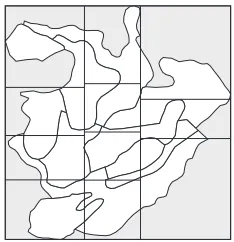
A trivial decomposition method is to use the compart-ments as the base for the decomposition and, without splitting compartments, assign each compartment to a process as in Figure 4. This approach has severe draw-backs: we couple the number of processes to the number of compartments, single compartment simulations are not parallelized, the workload is not evenly distributed but depends on the size of the compartment and it is hard to determine which processes need knowledge of a given tree.
Another well known method is to construct the bound-ing box of the simulation area and divide it into a grid with M·N cells, as shown in Figure 5 (M = N = 3). The drawback which makes this approach inadequate is that the sizes of the subdomains vary (between 8,900 m2
and 68,800 m2 in our example) and thus the workload
is unevenly distributed. We are also limited to M·N processes.
The orthogonal recursive bisection(ORB) algorithm (Warren and Salmon 1993) decomposes the area by re-cursively splitting the area into two parts in the x and y direction, both with equal workload. Using this method we acquire an equal workload in all subdomains, visu-alized in Figure 6 for P = 8. The downside with this approach is thatP must be a power of two, 2N.
The decomposition method used in SPATE-HPC is a modification of the ORB method. We determine a process grid size X·Y to use, like in the bounding box case, and use that to divide the area into X sections in the x-direction. We then recurse for each x-section and divide it intoYi orthogonal sections. The result, as shown in Figure 7 (X =Yi= 3), consists of subdomains
with equal workload. By allowing the number of sub sections within the x-sections to vary we can actually use any number of processes with this method.
4.2 Determining the grid size The challenge in our modified decomposition algorithm is to determine X and Yi. Given X and Yi the algorithm is
determinis-tic and will create a decomposition with equal workload for each subdomain. The problem of determiningX and
Yi resembles the constrained matrix-matrix
multiplica-tion (MMM) problem (Beaumont et al. 2000) where a unit square is divided intoPnon-overlapping rectangles according to an area criteria si for each P such as to minimize the sum of the perimeters. With the addi-tional constraint that the tiling is made up of columns, exactly like in our method, the optimal solution can be calculated. We cannot directly take advantage of that method as the simulation area is not a rectangle and thus does not completely cover the bounding box.
Figure 4: The sample area decomposed using the compartments (P = 11). The optimal area for each subdomain is 31,970 m2 while the actual sizes
vary between 12,340 m2
and 64,000 m2.
Figure 5: The sample area decomposed using the bounding box, P = 9. The optimal area for each subdomain is 39,075 m2 while the actual sizes
vary between 8,900 m2
and 68,800 m2.
Figure 6: The sample area decomposed using the orthogonal recursive bisection method, P = 8. All subdomains have the optimal area 43,960 m2.
Figure 7: The sam-ple area decomposed us-ing the modified orthog-onal recursive bisection method, P = 9. All sub-domains have the optimal area 39,075 m2.
the sum of the perimeters and thus also the communi-cation overhead as the data that needs to be commu-nicated is proportional to the number of trees close to the border, which again is proportional to the length of the borders of the rectangle (l1,l2). The overhead for a subdomain is thusO= 2·l1+ 2·l2. The individual sub-domain has the shortest perimeter when it is a square and the minimum value for the sum of the perimeters is thus reached when all subdomains are square shaped.
To make the individual cells as close to squares as possible we use the aspect ratio (x/y) of the simulation area’s bounding box and the number of processes (P) to determineX andY. Denoting byZthe largest integer smaller than or equal toZ, we have
X =√P·x/y (6)
Y =√P·1.0
x/y (7)
TheX andY we calculate using eqs. 6 and 7 will not always utilize allPprocesses, i.e. X·Y =P. Taking into account that the communication time in one time step is generally much smaller than the time needed to perform the calculations within a subdomain we obviously want to utilize all available processes. To be able to do this we disregard the communication overhead and trim the larger of X and Y up until we reach X and Y values such thatX·Y≤P, (X+ 1)·Y > P andX·(Y + 1)> P. If we still haveX·Y < Pwe haveL=P−XY leftover processes with no place in the grid. We add these left-over processes to the x-sections, at most one in each sec-tion, and introduce an additional communication over-head proportional to the width of the affected sections.
Figure 8: The sample area decomposed for 11 processes. The size of each subdomain is equal even though the first two x-sections contain an additional process, that is, four processes instead of three.
TheYi value for the firstL x-sections will then be one
larger than the otherYivalues. A decomposition of the sample area (Figure 1) with 11 processes thus produces the configuration in Figure 8.
4.3 Implementing the process decomposition
grid Each process can, provided with basic information on the system (number of processes, own id, simulation area), calculate its position in the decomposition grid independently of the other processes. The first step is to determine the number of rows and columns in the de-composition (X andY) using eq. 6 and eq. 7. Based on this, the process can calculate its position (x, y) in the process grid using x = P IDY , y = P IDmodY, where
bound-aries using the modified recursive algorithm. As the re-cursion is limited to two levels the calculation time is independent of the number of processes in the system. Taking into account the possibility of leftover processes in the firstLx-sections the fraction of the workload that should be on the left side of both boundary locations re-spectively can be calculated. Using a binary search and the calculated fractions the process finds the start and the end of the x-section which it is part of.
Once the x-boundaries are known the y-boundaries can be calculated in a similar manner by dividing the x-section into as many parts as there are processes in the section (Yi) and use another binary search to locate the
boundaries where the workload above and below corre-spond to the number of processes above and below.
4.4 Neighbors and communication To be able to communicate with other processes, each process must be aware of which processes are its neighbors and which borders they have in common. As the grid is not regu-lar, a process cannot without calculating all processes’ boundaries by itself determine which processes are its neighbors, or even how many neighbors it has. Typically a process in a large grid has 8 neighbors (the surround-ing cells). In SPATE-HPC the processes broadcast their coordinates once they have been calculated. The other processes pick up the information and determine which border (if any) is common to both. Two processes are neighbors even if they are not physically connected to each other but the distance between two points in each of the areas is less than the competition distance.
As all calculations during one simulation time step are based on the state at the beginning of the time step, we only need to communicate tree information once per time step. At the beginning of each time step we send information about all trees which are less than the com-petition distanceCaway from a cell border. If the com-petition distance is tree dependent we can use the largest competition distance asC. Information about different trees needs to be sent to different cell neighbors, depend-ing on which borders the processes share. For a neighbor to the right we consider the trees along the right border, for a neighbor below the bottom border, etc. The total number of trees for which data must be sent is usually very small compared to the total number of trees in each process.
5
Load balancing
The initial domain decomposition is well balanced pro-vided that the forest is and stays equidense. This is a good approximation for a small forest area where no management is performed. In a larger simulation area there will inevitably be denser and sparser
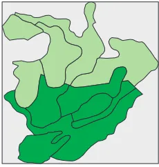
compart-Figure 9: The sample area covered with roughly 50% dense (darker) forest and 50% sparse (lighter) forest.
ments. Harvesting a large part of the forest in one time step will also alter the density and lessen the workload for some processes until new seedlings have grown. We deal with these load balancing problems by rebalancing the system as needed.
We rebalance the system by performing a new domain decomposition, identical to the one performed at the ini-tial stage of the simulation but using a more complete workload formula. At this point we have tree informa-tion and can thus include density in the workload calcu-lations. The time needed to simulate one time step for one part of the forest with N trees andD trees/m2 is
given in eq. 5. Disregarding the communication timeO we see that the workload is proportional toN·D.
Using N·D as weight we perform the decomposition and take trees and density into account to achieve a better balance. We still assume equal density within the compartments and calculateN andDper compartment. For a partial compartment we calculate the fraction of the area which is inside the subdomain and use that to calculateN andD.
The sample area from Figure 1 with roughly 50% of the compartments covered with sparse forest (1,100 trees/ha) and roughly 50% covered with dense forest (2,100 trees/ha), as illustrated in Figure 9, demonstrates a case where the initial load balance is skewed. Figure 10 shows the execution time for the individual processes per time step when using 8 processes. The processes with the most work are doing three times as much work as the processes with the least work. By rebalancing the simulation after the first time step (in which trees are generated), we acquire a much better balance. This is shown in Figure 11. Figure 12 shows how the process borders move in the rebalancing operation.
Figure 10: Process load balance for the area in Figure 9 when rebalancing is not used.
Figure 11: Process load balance for the area in Figure 9 when rebalancing is used. Rebalance overhead is shown as a darker area.
placed in memory in each process.
The time needed for time step 2 includes an rebalanc-ing overhead of two seconds, but still the execution time for the time step is more than 5 seconds less compared to the case where no balancing is done. In time step 3 and subsequent time steps the rebalance overhead is much smaller and thus the gain is even greater.
We check for load balancing problems at the begin-ning of every time step. We calculate the current weight (N·D) for each process and then the difference between the maximum and minimum weight in the system. If the difference is larger than a user given percentage, we perform a rebalancing operation. The weight calculation operation introduces a small overhead in each time step, seen for time step 3 in Figure 11. This overhead is several times smaller than the overhead for the actual rebalanc-ing operation but in naturally balanced cases it pays off to disable the rebalancing operations completely.
6
Validation of the parallel version
We have compared the results of the parallel version of SPATE-HPC to a sequential version in order to ensure
Figure 12: Rebalancing the area moves process borders towards the denser parts.
that the parallel version takes all boundary cases into account and otherwise also behaves as expected. The random numbers used in the simulation make it impos-sible to directly compare the raw tree data output (loca-tions and properties) between the versions. In a parallel simulation, the random numbers are generated individ-ually in each process using the parallel random number generator (Mascagni and Srinivasan 2000) to ensure in-dependent random numbers in each process. Because of this, the random tree locations will differ between a sequential and a parallel run, and also between two parallel runs with a different number of processes. The statistical output summary can be compared by hand in all cases but only to the extent that it is similar, not ex-actly the same. To verify the correctness of the parallel implementation we have included a special mode in the program that ensures that the random numbers are the same for each individual tree independent of how many processes are used in the simulation.
to changing the seed in a normal simulation so we are not limited to validating a single test case. We have used this method to validate that the parallel version of SPATE-HPC produces exactly the same results as the sequential version.
7
Performance
We have used a simulation area of 32,300 hectares containing 253 compartments in order to measure the scalability of SPATE-HPC. The size of the area was cho-sen in such a way that the same tests could be run on 32 and 2,048 cores using no more than 1GB of memory per core. The test case has been executed on a Cray XT4/XT5 hybrid machine with 2.3GHz quad-core pro-cessors and on an AMD cluster with 2.6GHz dual-core processors. Up to 2,048 cores were used on the Cray and up to 256 cores on the cluster.
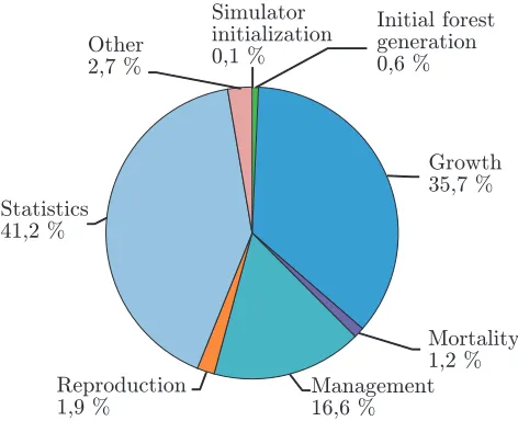
The performance of SPATE-HPC was measured by timing the execution of the full program (wall clock time) including all input and output phases. A break-down of the run time for a 110 time step simulation performing growth, mortality, reproduction and selec-tive thinning (every 15 time steps) on a 59 ha area using a single processor can be seen in Figure 13. The major-ity of the run time (53%) is spent in the time steps, in this case mostly in the growth part. A large part of the time (41%) is also spent on gathering statistics during the time steps and summarizing them at the end of the simulation.
Figure 13: Run time breakdown for a 59 ha case on one processor.
The parallel version of the program scales superlin-early with a speedup factor of 10.4 between 32 and 256 cores (linear=8) and 88.6 between 32 and 2,048 cores
(linear=64) as shown in Figure 14. The AMD cluster performs slightly worse but still exhibits almost linear scaling with a factor of 7.6 between 32 and 256 cores (expected=8). The superlinearity on the Cray is possi-ble due to better cache usage when the amount of data stored in each core decreases. A smaller simulation area in each core also implies that the cache is more efficiently used when locating neighboring trees due to data local-ity.
Figure 14: Scalability test on 32-2,048 cores for a fixed simulation area. Y-axis show the speedup (wall clock time) compared to 32 cores.
To verify that the program can simulate very large areas we have also investigated the scalability when the simulation area per core is kept constant, i.e. increas-ing the size of the total simulation area when increasincreas-ing number of cores. In the ideal case we would be able to double the simulation area, double the number of cores and complete the simulation in the same wall clock time as before. SPATE-HPC does not in this sense scale per-fectly but as Figure 15 shows, the required time for the simulation does not increase more than 30% on the Cray even when making the simulation area 64 times larger (32 cores vs. 2,048 cores).
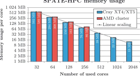
To be able to simulate very large areas it is not suf-ficient that the program scales performance-wise very well, but it must also be able to efficiently utilize the memory available in each process. We have measured the memory usage for the scalability test case in Fig-ure 14. Memory usage has been measFig-ured by sampling in all cores throughout the simulation. The value that represents the memory usage is the maximum amount used in any core at any point in time. The results of the measurements can be seen in Figure 16.
Figure 15: A simulation on 32-2,048 cores with fixed tree density and an increasing simulation area of 1,000ha/core.
Figure 16: Maximum memory usage per core for a fixed case using different number of cores. MPI overhead and static memory usage in SPATE-HPC have been excluded from this figure.
introduces an additional MPI overhead of 75MB in each core independent of the number of cores used, while the AMD cluster introduces an overhead which is dependent of the number of coresC(roughly 0.5·CMB in each pro-cess). We have excluded both the MPI overhead and the static overhead from Figure 16, which shows the mem-ory scalability of the program. As can be seen from the figure the memory usage on both machines scales almost linearly with the number of cores.
8
Conclusions
We have described the parallelization of SPATE-HPC, a single tree level forest dynamics simulator capable of simulating trees in polygonal forest areas. We have also described the computational challenges in the program and shown how they have been efficiently solved both regarding to CPU and memory usage.
SPATE-HPC has been parallelized in such a way that single tree level simulations on a very large scale can be
performed. The same simulator and the same simula-tion models can also be used for small forest areas. We can scale up to a landscape scale and simulate forests of several million hectares or we can just as accurately simulate small forests of a few hectares.
The strength of SPATE-HPC lies in being able to use a large amount of individual tree data from forest invento-ries. Laser scanning and other remote sensing methods have potential to become more common and more accu-rate in the future. These methods could provide coarser tree aggregation type data which after refinement to sin-gle tree level data is usable as input for the simulator. The simulator output would then be directly mappable to the original forest area and could be used to make predictions about the future yield of the forest. Alter-natively, SPATE-HPC could be used as a management tool to estimate which trees to harvest in the current situation.
SPATE-HPC is available as open source from the research project web page at
http://www.it.abo.fi/suswood.
Acknowledgements
The facilities of CSC (IT Center for Science Ltd) were used for this work. This work received support from the Academy of Finland in the “Sustainable production and products” research programme KETJU. We would like to thank the reviewers of this article for their valuable comments.
References
Beaumont, O., V. Boudet, F. Rastello, and Y. Robert, 2000. Matrix-matrix multiplication on heterogeneous platforms. In 2000 International Conference on Par-allel Processing (ICPP’00), p. 289.
Buckland, M., 2004. Programming game AI by example. Jones and Bartlett Publishers.
Coligny, F. D., et al., 2003. Capsis: Computer-aided pro-jection for strategies in silviculture : Advantages of a shared forest-modelling platform. In Modelling forest systems. Reality, models and parameters estimation -the forestry scenario, pp. 320–323. CABI Publishing, Sesimbra, Portugal. Workshop on Reality, Models and Parameter Estimation, the Forestry Scenario.
Cybenko, G., 1989. Dynamic load balancing for dis-tributed memory multiprocessors. Journal of Parallel and Distributed Computing 7(2):279–301.
Gropp, W., E. Lusk, and A. Skjellum, 1999. Using MPI: Portable Parallel Programming with the Message-Passing Interface. MIT Press.
Harja, D., and G. Vincent, 2008. Sexi-fs: Spa-tially explicit individual-based forest simula-tor - user guide and software. World Agro-forestry Centre ICRAF, Bogor, Indonesia. http://www.worldagroforestry.org/.../SExI/ (last access date: Feb. 17, 2010).
Lin, C., 2003. Generating Forest Stands with Spatio-Temporal Dependencies. Ph.D. thesis, University of Joensuu.
Mascagni, M., and A. Srinivasan, 2000. Algorithm 806: Sprng: A scalable library for pseudorandom number
generation. ACM Transactions on Mathematical Soft-ware 26:436–461.
Porte, A., and H. Bartelink, 2002. Modelling mixed for-est growth: a review of models for forfor-est management. Ecological Modelling 150(1-2):141–188.
Pretzsch, H., P. Biber, and J. Dursky, 2002. The single tree-based stand simulator silva: construction, appli-cation and evaluation. Forest Ecology and Manage-ment 162:3–21.