Improved Algorithms for Predicting Polyadenylation Sites and Cell Membranes From Expression, Sequence, and Image Data

(1)

UC Riverside

UC Riverside Electronic Theses and Dissertations

Title

Permalink

https://escholarship.org/uc/item/87b0892h

Author

Arefeen, Ashraful

Publication Date

2019 Peer reviewed|Thesis/dissertation

(2)

UNIVERSITY OF CALIFORNIA RIVERSIDE

A Dissertation submitted in partial satisfaction of the requirements for the degree of

Doctor of Philosophy in Computer Science by Ashraful Arefeen September 2019 Dissertation Committee:

Dr. Tao Jiang, Chairperson Dr. Eamonn Keogh

Dr. Stefano Lonardi Dr. Vassilis Tsotras

(3)

Copyright by Ashraful Arefeen

(4)

The Dissertation of Ashraful Arefeen is approved:

Committee Chairperson

(5)

Acknowledgments

I like to express my gratitude to all who have influenced me in writing this dissertation. I am extremely greatful to my advisor, Dr. Tao Jiang, for his guidance, patience and suggestions during my graduate studies. I will always remember the weekly meetings with him during these five years. In those meetings, his critical comments and constructive suggestions worked as motivational boost. Special thanks to my committee members, Dr. Eamonn Keogh, Dr. Stefano Lonardi and Dr. Vassilis Tsotras for their valuable feedback and comments during my proposal defense. Moreover, I am thankful to Dr. Xinshu (Grace) Xiao for her valuable comments and guidance in my research. I would also like to thank Dr. Gaudenz Danuser and Dr. Satwik Rajaram for giving me the opportunities to work on some cool projects during my summer internship at UT Southwestern Medical Center.

Finally, I like to thank my parents and my wife, Fouzia Hossain Oyshi, for their constant support during the most difficult period of my life. Without them, this dissertation would not have been possible.

(6)

(7)

ABSTRACT OF THE DISSERTATION

by

Ashraful Arefeen

Doctor of Philosophy, Graduate Program in Computer Science University of California, Riverside, September 2019

Dr. Tao Jiang, Chairperson

Alternative polyadenylation (polyA) sites near the 30 end of a pre-mRNA creates

multiple mRNA transcripts with different 30 untranslated regions (30 UTRs). The sequence

elements of a 30 UTR are essential for many biological activities such as mRNA

stabil-ity, sub-cellular localization, protein translation, protein binding, and translation efficiency. Moreover, numerous studies in the literature have reported the correlation between diseases

and the shortening (or lengthening) of 30 UTRs. As alternative polyA sites are common in

mammalian genes, we develop two algorithms, named TAPAS and DeepPASTA, for pre-dicting polyA sites from different data: RNA-Seq expression and sequence data. TAPAS detects novel polyA sites of a gene from RNA-Seq reads by considering read coverage as a time series data. The method is then extended to identify polyA sites that are expressed

differently between two biological samples and genes that contain 30 UTRs with

shorten-ing/lengthening events. On the other hand, DeepPASTA predicts polyA sites from sequence and RNA secondary structure data using a deep learning framework. As polyadenylation is

(8)

can predict the most dominant (i.e., frequently used) polyA site of a gene in a specific tissue and relative dominance when two polyA sites of the same gene are given. Our extensive experiments demonstrate that both TAPAS and DeepPASTA significantly outperform the existing tools in polyA site analysis.

The cells and their internal organelles carry genetic information in all living organ-isms. An effective method of studying cells and their organelles at different timestamps is to analyze the fluorescent microscopic images of tissues. As a result, computer-automated analyses of such microscopic images are getting popular for their efficiency and minimal human interaction. One of the most important computer-automated analyses is the cell membrane prediction from cell nucleus data. We propose a new tool, named DeepCEP, to predict cell membranes from nuclei using the fluorescent microscopic image data. Our experiments demonstrate that DeepCEP can be a potentially useful tool for analyzing mi-croscopic images in practice.

(9)

List of Figures

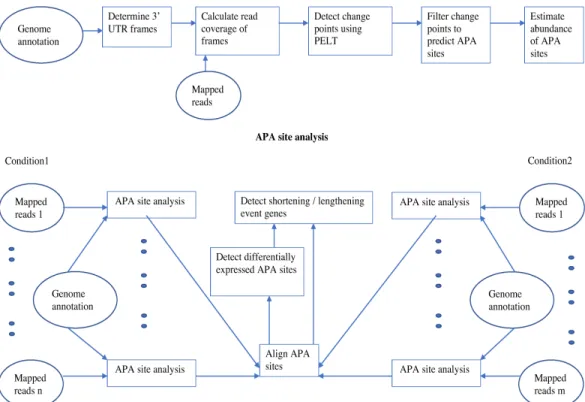
2.1 A flowchart of the TAPAS pipeline. In the differential expression analysis,

we assume that n RNA-Seq replicates are given for each condition. In the

figure, mapped reads also include read coverage information. . . 14

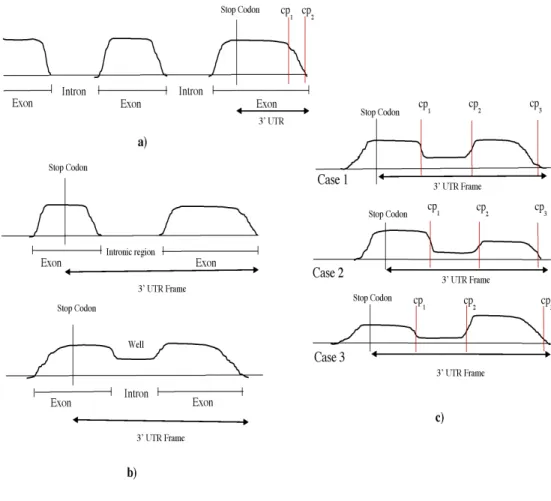
2.2 Some examples of filtration. (a) The PELT algorithm might output cp1 as

a change point even though the true APA site is cp2, which is removed by

TAPAS. (b) If a 30UTR frame contains an intron (either annotated or novel),

then a well might be created in the read coverage. (c) Three situations of the read coverage over the frame are illustrated. In case 1, the mean read coverages before and after the well are similar and TAPAS removes both

change pointscp1 andcp2around the well. In case 2, the mean read coverage

before the well is greater than the mean read coverage after the well and

TAPAS keeps cp1 as a potential APA site. In case 3, when the mean read

coverage before the well is smaller than that after the well (which is not

common), TAPAS would remove both change points as in the first case. . . 17

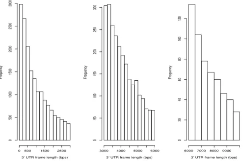
2.3 Length distribution of the 30 UTR frames extract from the human RefSeq

annotation GRCh37. The 30 UTR frames have lengths ranging from 2 bps

to 238,767 bps, with the average being 1,770.786 bps. . . 24

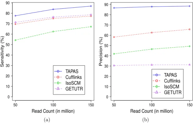
2.4 Performance of the tools in APA site detection on simulated data with

dif-ferent sequencing depths. Plot (a) shows the sensitivity and plot (b) shows

the precision. . . 25

2.5 Number of correct APA sites detected by different tools on the real dataset

when the flexible range for matching a predicted APA site to a true APA site

of 30-Seq is 50 bps (a) and 100 bps (b). . . 27

2.6 Performance of TAPAS, Cuffdiff, DESeq, and DEXSeq in differential

expres-sion analysis in terms of sensitivity (a) and preciexpres-sion (b). Cuffdiff anno de-notes running Cuffdiff with the transcriptome annotation and DEXSeq gene

denotes running DEXSeq to detect DE genes (instead of DE APA sites). . . 32

2.7 Performance of TAPAS, DaPars and ChangePoint on detecting genes with

(12)

3.1 The input and output of the polyA site prediction and tissue-specific polyA site prediction models of DeepPASTA. a) The polyA site prediction model of DeepPASTA takes a genomic sequence of 200 nts and three energy efficient RNA secondary structures predicted by RNAshapes [108] from the sequence as the input and predicts whether the input sequence contains a polyA site at the middle or not. b) Similar to the previous model, the tissue-specific polyA site prediction model of DeepPASTA takes a sequence and three cor-responding secondary structures generated by RNAshapes as the input and predicts whether the input sequence contains a polyA site at the middle or

not for the nine tissues studied in [31]. . . 52

3.2 The input and output of the tissue-specific relatively and absolutely

dom-inant polyA site prediction models of DeepPASTA. a) The tissue-specific relatively dominant polyA site prediction model of DeepPASTA takes a cou-ple of sequences and corresponding secondary structures containing polyA sites of some gene at the middle as the input and predicts which polyA site is relatively dominant. b) Unlike the relatively dominant model, the absolutely dominant model of DeePASTA takes a sequence and corresponding secondary structure containing a polyA site of some gene at the middle as the input and predicts whether the polyA site is an absolutely dominant polyA site of

the gene. . . 53

3.3 Architectures of the polyA site prediction model of DeepPASTA, M3 and

M4. The polyA site prediction model has four sub-models: a sequence and three secondary structure sub-models. Each sub-model consists of a

con-volution layer, a maxpooling layer, a recurrent layer (i.e., a bi-directional

LSTM), a flattening layer, and a fully connected layer. On the other hand, M3 (model represented by the red dotted line) consists of a sequence sub-model. M4 (model represented by the yellow dotted line) is similar to M3,

but its sequence sub-model does not contains a recurrent layer. . . 55

3.4 The training phase of the polyA site prediction model of DeepPASTA. In

each iteration of the training phase, the model predicts a likelihood value for the given input. This prediction is compared with the ground truth using a loss function. The loss value is then used to tune the parameters of the deep

learning model. . . 57

3.5 Architecture of the tissue-specific polyA site prediction model of DeepPASTA.

Similar to the polyA site prediction model of DeepPASTA, this model has a sequence and three secondary structure models. Each of these sub-models consists of a convolution layer, a maxpooling layer, a recurrent layer, a flattening layer, and a fully connected layer. This model is a multi-label classification model that has nine neurons in the output layer for predicting

(13)

3.6 Architecture of the model of DeepPASTA for predicting relative dominance in a particular tissue. The model takes two sequences of 200 nts and cor-responding secondary structures generated by RNAshapes containing polyA sites of some gene at the middle as the input. Each of these sequences and secondary structures is processed by a sub-unit, which consists of a sequence and a secondary structure sub-models. The output layer compares the

out-puts from the two sub-units to predict the relatively dominant polyA site. . 61

3.7 Architecture of the model of DeepPASTA for predicting absolutely dominate

polyA sites of each gene in a particular tissue. The model has a sequence and a secondary structure sub-models. The output layer predicts whether

the input polyA site is an absolutely dominant polyA site or not. . . 63

3.8 The impact of negative examples on the performance of DeepPASTA. In

order to test the performance of DeepPASTA in predicting polyA sites on different negative examples, three datasets are considered: datasets with shifted negative examples where positive examples are shifted left and right by 50 bases, with random negative examples that do not contain the hexamer signal and with random negative examples containing the hexamer signal. The positive examples of these datasets are the same.The number of examples for these three datasets are 286218, 190812 and 190744, respectively.Plots in a show the AUC and AUPRC performance of of DeepPASTA on the dataset with the shifted negative examples.Plots in b show the AUC and AUPRC performance on the dataset with the random examples that do not contain the hexamer signal.Plots in c show the AUC and AUPRC performance on

the dataset with the negative examples containing the hexamer signal. . . . 70

3.9 The RNA secondary structures of genes COX4I1 and ADORA2B helped

DeepPASTA in predicting polyA sites. The figure shows the secondary struc-tures generated by RNAshapes for the 100-nt upstream sequences of some polyA sites of the genes. Both polyA sites have AATAAA as the polyadeny-lation signal (PAS), but the locations of the signal in each input are far away from the polyA sites (the PASs and the polyA sites are colored red in the sequences). It is well known that the PAS often occurs 10-30 nts upstream of a polyA site ([46], [31] and [111]). Hence, one might conjecture that a PAS has to be near a polyA site in order for it to be functional. The folding of the RNA secondary structures reduces the distance between the PAS and polyA

(14)

3.10 Hexamer signals extracted from the true positive polyA sites predicted by DeepPASTA on dataset 1. In order to identify the most frequently used sig-nals, we consider the top three high strength 6-mers in each input sequence based on saliency maps. The barplot on the left shows the overall 20 most fre-quently used hexamer signals in polyA site prediction. Most of these signals are annotated in the literature [46], [31] and [111]. In addition, DeepPASTA used some novel hexamer signals: UAAAAU, GAAUAAA, UAAAUA, AAU-UAA, and UUAAAA. The four barplots on the right show the most frequently used hexamer signals in four equally divided regions (as illustrated at the bot-tom of the figure) of the input sequence. From the four barplots, it is seen that DeepPASTA used fewer signals from the fourth region (150-200 nts) in polyA site prediction. Similar to previous studies, DeepPASTA identified the U-rich signals as auxiliary upstream elements (AUEs) in the first region (1-49 nts), U/GU-rich signals as downstream elements in the third region (101-149 nts) and G-rich signals as auxiliary downstream elements (ADEs)

in the fourth region (150-200 nts). . . 72

3.11 Hexamer signals extracted from the true positive polyA sites predicted by the tissue-specific model of DeepPASTA on dataset 1 for the brain tissue. In order to identify the most frequently used signals, we consider the top three high strength 6-mers in each input sequence based on saliency maps. The barplot on the left shows the overall 20 most frequently used hexamer signals in polyA site prediction for the brain tissue. The four barplots on the right show the most frequently used hexamer signals in four equally divided regions (as illustrated at the bottom of the figure) of the input sequence. From these four barplots, it is seen that DeepPASTA used the most hexamer signals from the second region (50-100 nts) in polyA site prediction for the brain tissue. The most frequently used signals in that region are AAUAAA, AAAAAA, AAAAAG, AAAUAA, and CAAUAA. These signals are known

as the polyadenylation signals (PASs) in the literature [46], [31] and [111]. . 78

3.12 Hexamer signals extracted from the true positive polyA sites predicted by the tissue-specific model of DeepPASTA on dataset 1 for the kidney tissue. In order to identify the most frequently used signals, we consider the top three high strength 6-mers in each input sequence based on saliency maps. The barplot on the left shows the overall 20 most frequently used hexamer signals in polyA site prediction for the kidney tissue. The four barplots on the right show the most frequently used hexamer signals in four equally divided regions (as illustrated at the bottom of the figure) of the input sequence. From these four barplots, it is seen that DeepPASTA used the most hexamer signals from the second region (50-100 nts) in polyA site prediction for the kidney tissue. The most frequently used signals in that region are AAUAAA, AUAAAA, AAAUAA, AUAAAG, and CAAUAA. Again, these signals are known as the

(15)

3.13 Hexamer signals extracted from the true positive polyA sites predicted by the tissue-specific model of DeepPASTA on dataset 1 for the liver tissue. In order to identify the most frequently used signals, we consider the top three high strength 6-mers in each input sequence based on saliency maps. The barplot on the left shows the overall 20 most frequently used hexamer signals in polyA site prediction for the liver tissue. The four barplots on the right show the most frequently used hexamer signals in four equally divided regions (as illustrated at the bottom of the figure) of the input sequence. From these four barplots, it is seen that DeepPASTA used the most hexamer signals from the second region (50-100 nts) in polyA site prediction for the liver tissue. The most frequently used signals in that region are AAUAAA, AUAAAA, AAAUAA, AUAAAG, and AUUAAA. Again, these signals are known as the polyadenylation signals (PASs) in the literature [46], [31] and

[111]. . . 80

3.14 Hexamer signals extracted from the true positive polyA sites predicted by the tissue-specific model of DeepPASTA on dataset 1 for the MAQC Brain1 tissue. In order to identify the most frequently used signals, we consider the top three high strength 6-mers in each input sequence based on saliency maps. The barplot on the left shows the overall 20 most frequently used hexamer signals in polyA site prediction for the MAQC Brain1 tissue. The four barplots on the right show the most frequently used hexamer signals in four equally divided regions (as illustrated at the bottom of the figure) of the input sequence. From these four barplots, it is seen that DeepPASTA used the most hexamer signals from the second region (50-100 nts) in polyA site prediction for the MAQC Brain1 tissue. The most frequently used signals in that region are AAUAAA, AAAUAA, AUAAAA, AUUAAA, and AUAAAG. Again, these signals are known as the polyadenylation signals (PASs) in the

literature [46], [31] and [111]. . . 81

3.15 Hexamer signals extracted from the true positive polyA sites predicted by the tissue-specific model of DeepPASTA on dataset 1 for the MAQC Brain2 tissue. In order to identify the most frequently used signals, we consider the top three high strength 6-mers in each input sequence based on saliency maps. The barplot on the left shows the overall 20 most frequently used hexamer signals in polyA site prediction for the MAQC Brain2 tissue. The four barplots on the right show the most frequently used hexamer signals in four equally divided regions (as illustrated at the bottom of the figure) of the input sequence. From these four barplots, it is seen that DeepPASTA used the most hexamer signals from the second region (50-100 nts) in polyA site prediction for the MAQC Brain2 tissue. The most frequently used signals in that region are AAUAAA, AAAUAA, AUAAAG, CAAUAA, and UAAUAA. Again, these signals are known as the polyadenylation signals (PASs) in the

(16)

3.16 Hexamer signals extracted from the true positive polyA sites predicted by the tissue-specific model of DeepPASTA on dataset 1 for the MAQC UHR1 tissue. In order to identify the most frequently used signals, we consider the top three high strength 6-mers in each input sequence based on saliency maps. The barplot on the left shows the overall 20 most frequently used hexamer signals in polyA site prediction for the MAQC UHR1 tissue. The four barplots on the right show the most frequently used hexamer signals in four equally divided regions (as illustrated at the bottom of the figure) of the input sequence. From these four barplots, it is seen that DeepPASTA used the most hexamer signals from the second region (50-100 nts) in polyA site prediction for the MAQC UHR1 tissue. The most frequently used signals in that region are AAUAAA, AAAUAA, AUAAAA, AUUAAA, and UAAUAA. Again, these signals are known as the polyadenylation signals (PASs) in the

literature [46], [31] and [111]. . . 83

3.17 Hexamer signals extracted from the true positive polyA sites predicted by the tissue-specific model of DeepPASTA on dataset 1 for the MAQC UHR2 tissue. In order to identify the most frequently used signals, we consider the top three high strength 6-mers in each input sequence based on saliency maps. The barplot on the left shows the overall 20 most frequently used hexamer signals in polyA site prediction for the MAQC UHR2 tissue. The four barplots on the right show the most frequently used hexamer signals in four equally divided regions (as illustrated at the bottom of the figure) of the input sequence. From these four barplots, it is seen that DeepPASTA used the most hexamer signals from the second region (50-100 nts) in polyA site prediction for the MAQC UHR2 tissue. The most frequently used signals in that region are AAUAAA, AAAUAA, AUUAAA, AUAAAA, and UAAUAA. Again, these signals are known as the polyadenylation signals (PASs) in the

literature [46], [31] and [111]. . . 84

3.18 Hexamer signals extracted from the true positive polyA sites predicted by the tissue-specific model of DeepPASTA on dataset 1 for the muscle tissue. In order to identify the most frequently used signals, we consider the top three high strength 6-mers in each input sequence based on saliency maps. The barplot on the left shows the overall 20 most frequently used hexamer signals in polyA site prediction for the muscle tissue. The four barplots on the right show the most frequently used hexamer signals in four equally divided regions (as illustrated at the bottom of the figure) of the input sequence. From these four barplots, it is seen that DeepPASTA used the most hexamer signals from the second region (50-100 nts) in polyA site prediction for the muscle tissue. The most frequently used signals in that region are AAUAAA, AUUAAA, AAAUAA, AUAAAA, and AUAAAG. Again, these signals are known as the

(17)

3.19 Hexamer signals extracted from the true positive polyA sites predicted by the tissue-specific model of DeepPASTA on dataset 1 for the testis tissue. In order to identify the most frequently used signals, we consider the top three high strength 6-mers in each input sequence based on saliency maps. The barplot on the left shows the overall 20 most frequently used hexamer signals in polyA site prediction for the testis tissue. The four barplots on the right show the most frequently used hexamer signals in four equally divided regions (as illustrated at the bottom of the figure) of the input sequence. From these four barplots, it is seen that DeepPASTA used the most hexamer signals from the second region (50-100 nts) in polyA site prediction for the testis tissue. The most frequently used signals in that region are AAUAAA, AUAAAA, AAAUAA, AUAAAG, and AUUAAA. Again, these signals are known as the polyadenylation signals (PASs) in the literature [46], [31] and

[111]. . . 86

3.20 Number of examples in the training and validation data used in the experi-ments on predicting tissue-specific relatively dominant polyA sites. As shown in the left plot, the number of training examples in dataset 4 ranges from 59.4% to 64.3% of the total number of examples (used in training, validation and testing) across all tissues, and the number of validation examples ranges from 15.8% to 19.7%. As shown in the right plot, the numbers of training and validation examples range from 60.5% to 61.7% and from 22.3% to 22.8%,

respectively. . . 88

3.21 Number of examples in the training and validation data used in the exper-iments on predicting tissue-specific absolutely dominant polyA sites of each gene. As the plot shows, the number of examples in the training data ranges from 54.1% to 55.9% and the number of examples in the validation data

ranges from 22.6% to 23.4%. . . 91

4.1 The input and output of the filtering and main models of DeepCEP. a-b)

The filtration model of DeepCEP takes a patch containing three channels (nucleus, stroma, and cell structure) as the input and predicts better cell structure containing patches. These patches works as the ground truth data of the main model. c-d) The main model of DeepCEP takes a patch con-taining two channels (nucleus and stroma) as the input and predicts cell membanes of the input patch. More specifically, this model predicts the cell

membranes around the nuclei of the input patch. . . 100

4.2 Architecture of the filtration model. The model has three identical U-net

sub-models. The input to the model is a patch consisting of three channels: necleus, stroma and unfiltered cell structure strain channels. The output from the model is a patch consisting of filtered cell structure strain channel. Each of these U-net sub-models consist of multiple convolution layers to extract

features from the input patch. . . 103

4.3 Architectures of the Resnet and U-net sub-models of the cell structure model.

These sub-models consist of mulitple convolution layers to extract features

(18)

4.4 Architecture of the cell structure model. The cell structure prediction model has four models: a U-net model and three identical Resnet sub-models. The input to the model is a patch consisting of necleus and stroma strain channels. The output from the model is a patch consisting of cell

membranes around the nuclei. . . 106

4.5 Some of the patches of the training data. The patches from the first row are

the input patches of DeepCEP. These patches contain nucleus and stroma strain channels. The second row shows the unfiltered cell structure strain channel patches corresponding to the patches of first row. The third row shows the filtered cell structure strain channel patches corresponding to the patches of second row. The patches from the third row are the ground truth patches of DeepCEP. Note that the filtered patches are generated using the

filtration model of section 4.2.1. . . 111

4.6 Performance comparison of DeepCEP and the baseline model for predicting

cell membranes from nuclei. a) Some of the input patches from Dataset 1. Each of these patches consists of two channels: nucleus and stroma strain channels. b) Expert’s annotation of cell membranes for these input patches. c) When the input patches are given to DeepCEP, it predicts the cell mem-branes. d) Similar to DeepCEP, when the input patches are given to the

(19)

List of Tables

2.1 Performance comparison in APA site detection on simulated data. The

num-ber of true APA sites is 21731. . . 26

2.2 Performance comparison in APA site detection on real data. Two flexible

ranges (50 bps and 100 bps) are considered for matching a predicted APA

site with a true one from 30-Seq. . . 28

2.3 Performance comparison in APA site detection on real data, when the

predic-tion results of the tools compared are filtered by the 30 UTR frames defined

by TAPAS. Two flexible ranges (50 bps and 100 bps) are considered for

matching a predicted APA site with a true one from 30-Seq. The number of

predicted APA sites of TAPAS is lowered to be closer to those of Cufflinks’ and IsoSCM’s. For a further comparison, Cufflinks is run with the reference

transcriptome in RefSeq (i.e., Cufflinks -g). Note that, given the number of

APA sites predicted by Cufflinks -g, its performance should be directly com-pared with that of TAPAS provided in Table S2 rather than the numbers in

this table. . . 28

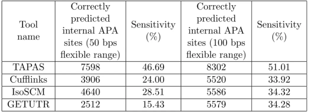
2.4 Performance comparison in detecting internal APA sites located inside the

30 UTR frames on real data. . . 29

2.5 Performance comparison in APA site detection on real data. Two flexible

ranges (50 bps and 100 bps) are considered for matching a predicted APA

site with a true one from PAS-Seq. . . 29

2.6 Performance comparison in the detection of genes with differentially

ex-pressed (DE) APA sites on simulated data. The number of genes with actual DE APA sites is 1254, and each such gene contains only one DE APA sites. Since DEXSeq is designed for differential splicing (DS) rather than DE anal-ysis [76, 104], we consider DE genes with at least two transcripts (298 in total) as the benchmark when evaluating the performance of DEXSeq. Here,

Cuffdiff anno = Cuffdiff with annotation. . . 34

2.7 Performance comparison in the detection of genes with shortening/lengthening

events on simulated data. The actual number of genes with shortening/lengthening

events is 674. . . 38

2.8 Performance comparison in the detection of genes with shortening/lengthening

(20)

2.9 Performance comparison between TAPAS and 3P-Seq in APA site detec-tion on mouse liver data. Paired-end RNA-Seq reads from standard polyA+ libraries for mouse liver (SRX196268) were downloaded from NCBI and mapped by TopHat2 to the mouse genome. For performance evaluation,

a 30-Seq dataset for mouse liver (GSM747483) was also downloaded from

NCBI and used as benchmark. We ran TAPAS on the mapped reads and compared its predicted APA sites against the benchmark. As a comparison, we downloaded the 3P-Seq data for mouse liver (GSM1268948) from NCBI. Among the 29932 APA sites reported in the 3-Seq data, TAPAS and 3P-Seq identified 10900 and 19480 sites, respectively. In terms of sensitivity, 3P-Seq outperforms TAPAS; but TAPAS outperforms 3P-Seq in terms of precision. Note that TAPAS uses standard RNA-Seq data which is very popular and easy to perform while 3P-Seq requires complex biological steps and large

amounts of RNA for its analysis [55]. . . 40

2.10 Comparison of time (in minutes) and peak memory (in gigabytes) usage among the APA site detection tools on the simulated dataset with 50 million reads used in Section 2.3.1. Here, the running time of TAPAS includes the

calculation of read coverage by SAMtools. . . 41

2.11 Comparison of time and peak memory usage among the tools for shorten-ing/lengthening analysis on the simulated dataset with 50 millions reads used in Section 2.3.3. Again, the running time of TAPAS includes the calculation

of read coverage by SAMtools. . . 42

3.1 Performance comparison between DeepPASTA, PolyAR, Dragon PolyA

Spot-ter, DeeReCT-PolyA, Conv-Net, and DeepPolyA in polyA site prediction on the three datasets introduced in the beginning of section 3.3.1 in terms of

AUC and AUPRC. . . 68

3.2 The effect of data leak on DeepPASTA in polyA site prediction on dataset 1

in terms of AUC and AUPRC. . . 73

3.3 Contributions of the RNN and RNA secondary structures in polyA site

pre-diction on datasets 1 and 2 in terms of AUC and AUPRC. . . 74

3.4 Performance comparison between the tissue-specific model of DeepPASTA,

DeepPolyA and basic (i.e., non-tissue-specific) polyA site prediction models

of DeepPASTA on datasets 1and 2. Table S1 of the Supplementary Materials shows the numbers of positive and negative examples in the test datasets.

Datasets 1 and 2 are represented as D1 and D2, respectively, in the table. . 76

3.5 Performance comparison between DeepPASTA and Conv-Net in relatively

dominant polyA site prediction on dataset 4 in terms of AUC and AUPRC. The performance of Conv-Net is based on our implementation of the method

described in [68] . . . 89

3.6 Performance comparison between DeepPASTA and Conv-Net [68] in

(21)

3.7 Performance comparison between DeepPASTA and Conv-Net in predicting absolutely dominant polyA sites on dataset 6 in terms of AUC and AUPRC.

The 2nd and 3rdcolumns give the number of positive and negative examples

in the test data. . . 91

3.8 Training time of the four DeepPASTA models in our experiments. . . 93

4.1 Performance comparison between DeepCEP and the baseline model in

pre-dicting cell from nuclei on Dataset 1 in term of sensitivity and precision. Dataset 1 contains 20 annotated patches, and there are 639 cells in these

patches. . . 115

4.2 Performance comparison between DeepCEP and the baseline model in

pre-dicting cell from nuclei on Dataset 2 in term of sensitivity and precision. Dataset 2 contains 12000 patches, and there are 137058 cells in these patches. 115

(22)

Chapter 1

Introduction

1.1 Polyadenylation site analysis

According to the central dogma of molecular biology, a DNA sequence is converted to proteins using transcription, post-transcriptional, and translation processes. Initially, the transcription process synthesizes a mRNA from a fragment of DNA [65]. This pre-mRNA is converted to a mature pre-mRNA by the post-transcriptional process. Finally, the mature mRNA is translated into the corresponding protein. There are three important steps

in the post-transcriptional process [58]: addition of a 50 cap, addition of a polyadenylation

(polyA) tail, and splicing. The polyA tail is added to the 30 end of a pre-mRNA by the

polyadenylation process. More precisely, the polyadenylation process consists of two steps

[120]: cleavage near the 30 end of a pre-mRNA and the addition of a polyA tail at the

cleavage site.

A 30 untranslated region (UTR) is a suffix of an mRNA that starts after the stop

(23)

30 end of an pre-mRNA create more than one mRNA transcripts containing 30 UTRs of

different lengths. The length of a 30 UTR and the sequence elements (such as those AU and

GU rich elements) near a 30end may have an impact on mRNA stability, mRNA localization,

protein translation, protein binding, and translation efficiency [15]. Moreover, the secondary

structure of a 30UTR is also important for translation efficiency and disruption of expression

[15]. Alternative polyadenylation is very common phenomenon in eukaryote genes [111] and most human genes have alternative polyadenylation in their post-transcription process [81]. Therefore, the analysis of polyA sites would be of great importance in the study of mammalian genes.

1.1.1 Alternative polyadenylation site analysis from RNA-Seq expression data

The study of transcription has been advanced by the recent improvement in se-quencing technologies. The advent of next-generation sese-quencing (NGS) technologies [16] has drastically improved sequencing time and cost. RNA sequencing (RNA-Seq), also known as whole transcriptome shotgun sequencing [83], uses NGS to study the presence and ex-pression of an RNA in a biological sample in a given moment [27, 124]. RNA-Seq is an efficient way to track the continuously changing transcriptome. More specifically, RNA-Seq facilitates the ability to look at alternative spliced transcripts, post-transcriptional modifica-tions, gene fusion, mutations/SNPs, and changes in gene expression over time or differences in gene expression in different groups or treatments [78]. In addition to determining the

exon/intron boundaries in genes, RNA-Seq can be used to profile the 50 and 30 ends of

(24)

anal-ysis. Recently, several tools have been published for detecting APA sites from RNA-Seq data or performing shortening/lengthening analysis. These tools consider either up to only two APA sites in a gene or only APA sites that occur in the last exon of a gene, although a gene may generally have more than two APA sites and an APA site may sometimes oc-cur before the last exon. Furthermore, the tools are unable to integrate the analysis of shortening/lengthening events with APA site detection.

In chapter 2, we propose a new tool, called TAPAS, for detecting novel APA sites from RNA-Seq data. It can deal with more than two APA sites in a gene as well as APA sites that occur before the last exon. The tool is based on an existing method for finding change points in time series data, but some filtration techniques are also adopted to remove change points that are likely false APA sites. It is then extended to identify APA sites that are

expressed differently between two biological samples and genes that contain 30 UTRs with

shortening/lengthening events. Our extensive experiments on simulated and real RNA-Seq data demonstrate that TAPAS outperforms the existing tools for APA site detection and shortening/lengthening analysis significantly.

1.1.2 PolyA site analysis from sequence data

DNA is a molecule that carries genetic instructions for the development, func-tioning, growth, and reproduction of all known organism and many viruses. The instruc-tion/information in DNA is stored as a code made up of four chemical/nucleotide bases: adenine (A), guanine (G), cytosine (C), and thymine (T). Human DNA consists of about 3 billion bases, and the order of these bases is extremely important for carrying genetic instructions. DNA sequencing is the process of determining the order of these nucleotide

(25)

bases in DNA. Nowadays, DNA sequencing has become very crucial in numerous fields such as biotechnology, forensic biology, and medical diagnostics. The development of next-generation sequencing (NGS) technologies [16] has drastically improved sequencing time, cost, and efficiency. Moreover, these technologies have facilitated researchers in investi-gating insights into health, human origins, etc. Due to the advancement of sequencing technologies, computational tools are developed to analyze the sequence data. Selection of a polyadenylation site for the polyadenylation process also depends on the sequence motifs

orcis-elements. As a result, several machine learning tools have been published for

predict-ing polyA sites from sequence data or performpredict-ing relative and absolute dominant analyses. These tools either consider limited sequence features or use relatively old algorithms for polyA site prediction. Moreover, none of the previous tools consider tissue specific polyA site analysis and RNA secondary structures as a feature to predict polyA sites.

In chapter 3, we propose a new deep learning model, called DeepPASTA, for predicting polyA sites from both sequence and RNA secondary structure data. The model is then extended to predict tissue-specific polyA sites. Moreover, the tool can predict the most dominant (i.e., frequently used) polyA site of a gene in a specific tissue and relative dominance when two polyA sites of the same gene are given. Our extensive experiments demonstrate that DeepPASTA significantly outperforms the existing tools for polyA site prediction and tissue-specific relative and absolute dominant polyA site prediction.

(26)

1.2 Fluorescence microscopic image analysis for cell

mem-brane prediction

The cell is the basic building unit for all living organisms. The interior of a cell consists of different organelles, and one of the major organelles is the cell nucleus. The cell nucleus works as a repository of information for all living organisms. As cells and their organelles are very important, it is essential to various research areas to study cells and their sub-cellular components. One powerful way of studying cells and its organelles at different timestamps is to analyze the microscopic images of tissues. Fluorescence labeling on top of the microscopy imaging provides unprecedented opportunities to study the structural features and functional characteristics of a cell, e.g., cell nucleus, cell membrane, stroma, cell proliferation signal, etc. However, fluorescence labeling has some limitations. In order to overcome these limitations, computer-automated analyses on the microscopic images

are getting popular. Recently, several machine learning tools have been developed for

automatically analyzing the microscopic images. One of the most important automatic analyses is cell membrane prediction. Although there are several tools for cell membrane prediction, none of them predicts it only from the nucleus.

In chapter 4, we propose a new deep learning model, called DeepCEP, for predict-ing cell membranes from nuclei uspredict-ing the fluorescence microscopic image data. Our extensive experiments demonstrate that DeepCEP significantly outperforms a baseline model for cell membrane prediction.

(27)

1.3 Publications

This dissertation encompasses two publications. The TAPAS [10] paper (Chapter 2) is published in Bioinformatics journal (2018). The DeepPASTA [11] paper (Chapter 3) is also published in Bioinformatics journal (2019). The complete list of publications includes:

• Ashraful Arefeen, Juntao Liu, Xinshu Xiao and Tao Jiang. TAPAS: tool for alternative

polyadenylation site analysis. Bioinformatics, 2018, 34(15).

• Ashraful Arefeen, Xinshu Xiao and Tao Jiang. DeepPASTA: deep neural network

(28)

Chapter 2

TAPAS: tool for alternative

polyadenylation site analysis

2.1 Introduction

According to the central dogma of molecular biology, the transcription process in eukaryotes synthesizes a mRNA from the genomic sequence of a gene [65]. The pre-mRNA is then converted to a mature pre-mRNA by the post-transcriptional process. Finally, this mature mRNA is translated into the corresponding protein. The post-transcriptional

process includes three major steps: the addition of a 50 cap, addition of a polyadenylation

(polyA) tail and splicing. In particular, a polyA tail is added at the 30 end of a pre-mRNA

with the help of the polyadenylation process. More precisely, the polyadenylation process

consists of two steps [120]: cleavage near the 30 end of a pre-mRNA and the addition of a

(29)

been found in the literature that influence the choice of a particular polyA cleavage site

[15, 94]. In particular, the 30 end sequence of a pre-mRNA usually contains a AAUAAA

hexamer (or some close variant). This hexamer is called the polyadenylation signal (PAS) and it usually appears 10-30 bps upstream of the cleavage site [111]. The PAS serves as a binding site for the cleavage and polyadenylation specificity factor (CPSF). U-rich or U/G-rich elements located 20-40 bps downstream of the cleavage site are also involved in polyadenylation [111]. These U-rich or U/G-rich elements serve as the binding sites for the cleavage stimulation factor (CstF). In addition, some auxiliary elements upstream of the PAS and downstream of the cleavage site may enhance the polyadenylation process

[111]. Due to the interactions between these cis elements and polyadenylation factors,

alternative cleavage sites can be formed for a pre-mRNA, resulting in more than one mRNA

transcript from a single pre-mRNA containing 30 untranslated regions (30UTRs) of different

lengths. Note that a 30 UTR is a suffix of an mRNA sandwiched between the stop codon

and polyadenylation cleavage site of the mRNA. The length of a 30 UTR as well as some

sequence elements in the 30 UTR such as AU-rich elements and GU-rich elements may have

impact on mRNA stability, mRNA localization, protein translation, protein binding and

translation efficiency [15]. Moreover, the secondary structure of a 30 UTR is also important

for its translation efficiency and disruption of expression [15]. Alternative polyadenylation (cleavage) is very common in mammalian genes [111]. According to the study in [26], more than half of human genes have alternative polyadenylation in their post-transcriptional process. Therefore, the analysis of alternative (or all) polyadenylation sites (APA sites) would be of great importance for the study of mammalian genes.

(30)

The analysis of expressed sequence tags (ESTs) has provided genome-wide

anno-tations of 30 UTRs. Not only does this analysis show that mammalian genes have multiple

30 UTRs [111], but also it reveals that neuronal cell mRNAs have longer 30 UTRs than liver

cell mRNAs [106]. However, an EST based approach is not able to estimate the relative

abundance of each 30 UTR in the resultant mRNAs [55]. Using 3P-Seq data, the 30 UTRs

of genes in yeast, worm, fly, zebrafish, mouse and human genomes have been annotated in [48, 115, 85, 8, 79, 31, 45, 103]. Unlike EST based approaches, these methods based on

3P-Seq precisely detect the usage of different 30 UTRs in mRNAs. On the other hand, they

require complex biochemical steps and large amounts of RNA for their analyses [55]. The advancement of RNA-Seq technology has provided new avenues for the study of transcription including the polyadenylation process. A typical RNA-Seq data analysis process begins with mapping RNA-Seq reads to some reference genome using tools like TopHat2 [53], HISAT [54]. Once the reads are mapped, mRNA transcripts (or isoforms) are assembled by using tools like Cufflinks [113], IsoLasso [70], StringTie [93], or TransComb [75], and their abundance levels are quantified by using tools like Cufflinks [113], RSEM [69], CEM [71], eXpress [96], Kallisto [19], etc. Moreover, differential expression between samples can be analyzed by using tools such as DESeq [7], Cuffdiff [114] or DEXSeq [6].

Recently, several methods for discovering 30 UTRs from RNA-Seq data have been

introduced in the literature. The tool introduced in [77] studies the dynamic expression of 30

UTRs using a Poisson hidden Markov model. Due to the design of the model, the tool is only able to identify up to two alternative polyadenylation sites for a given gene. The web server

(31)

UTRs. It only reports the polyadenylation sites given in the transcriptome and thus would be unable to provide any novel APA sites. Roar [40] takes annotated APA sites from public

databases to identify genes undergoing regulation of 30 UTR length. Similar to 3USS, Roar

is unable to discover novel APA sites. GETUTR [55] is another RNA-Seq based tool to

estimate the 30 UTR landscape. The method takes mapped reads and a reference genome

as the input, and finds APA sites by using techniques to smooth read coverage including isotonic (or monotone) regression [63]. A drawback of the method is that these smoothing techniques may result in many false APA sites. On the other hand, although introns may

occur in 30 UTRs ([15], [17]), GETUTR does not consider intronic regions in its analysis

and thus often misses 30 UTRs that contain introns. IsoSCM [102] identifies alternative 30

UTRs based on a multiple change-point inference model. It first uses the (statistical) model to infer change points in a gene that exhibit sharp increase or decrease in read coverage. Then it employs some additional mathematical constraint to filter change points that are likely to be false APA sites. Similar to GETUTR, the method does not consider introns

inside a 30 UTR. DaPars [127] and ChangePoint [122] are tools for comparing APA sites

in two biological samples and detecting shortening/lengthening events. Both of these tools consider only two cleavage sites in their shortening/lengthening analysis, although a gene may have more than two APA sites.

In this chapter, we introduce a new tool, called TAPAS (i.e., Tool for Alternative

Polyadenylation site AnalysiS), for detecting novel APA sites from RNA-Seq data. It can

deal with more than two APA sites in a gene as well as 30 UTRs that contain intronic

(32)

change points in time series data [52], but some filtration techniques that take into account

special properties of RNA-Seq data and the exonic structures of the 30 UTRs of the same

gene are also employed to remove change points that are likely false APA sites. The tool is then extended to identify APA sites that are expressed differently between two biological samples with multiple replicates by using an elaborate algorithm to align APA sites from each replicate and standard statistical approaches for differential expression analysis such as the one in [7]. The differential expression analysis is further extended to identify genes

that have 30 UTRs with shortening/lengthening events.

To assess the performance of TAPAS, we have conducted extensive experiments on both simulated and real data and compared TAPAS with the above mentioned tools IsoSCM, GETUTR, DaPars and ChangePoint for APA site or differential expression analy-sis. Moreover, since a complete transcriptome provides full information about APA sites, we also include the most popular tool for transcriptome assembly, Cufflinks, and its correspond-ing tool for transcript-based differential expression analysis, Cuffdiff, in the comparison. As none of these existing tools are able to perform all three types of APA site and differen-tial expression analysis that TAPAS can do, we organize the comparison as three groups: (i) detection of APA sites (between TAPAS, IsoSCM, GETUTR, and Cufflinks), (ii) detec-tion of genes with differentially expressed APA sites (between TAPAS, Cuffdiff, DESeq, and DEXSeq), and (iii) detection of genes with shortening/lengthening events (between TAPAS, DaPars and ChangePoint). We exclude 3USS, Roar and the tool in [77] from the comparison because they are either unable to discover novel APA sites or seriously restricted. In the simulation experiments, the tools are compared in terms of sensitivity and precision. Based

(33)

on these two performance measures, TAPAS outperforms IsoSCM, GETUTR and Cufflinks

significantly in the detection of APA sites. When 30-Seq (or polyA-Seq) and PAS-Seq data

are considered as the ground truth in real data experiments, TAPAS is able to deliver more true APA sites than the other tools with a similar number of predicted APA sites. For the detection of genes with differentially expressed APA sites, TAPAS achieves a higher sensitivity than Cuffdiff and DEXSeq even though they are provided with an annotated transcriptome. Although its sensitivity is initially worse than that of DESeq, the gap de-creases rapidly with the increase of sequencing depth. While its precision is also higher than that of Cuffdiff without the transcriptome annotation and DEXSeq, it is slightly lower than that of Cuffdiff with the transcriptome annotation and lower than that of DESeq (but the gaps shrink as well with the increase of sequencing depth). In the shortening/lengthening event analysis, TAPAS outperforms significantly DaPars and ChangePoint on simulated

data. On a real dataset and once again using 30-Seq data as the ground truth, TAPAS

iden-tifies more genes with real shortening/lengthening events than the other two, when all the tools are tuned to output similar number of events. We also analyze the time and memory efficiency of TAPAS and demonstrate that while TAPAS requires a significant amount of memory, its running time is comparable to that of the other tools.

The rest of the chapter is organized as follows. The method of TAPAS is discussed in section 2.2. The experimental results and comparison with the other tools are given in section 2.3. A brief evaluation of the running time and memory efficiency of the tools is given in section 2.4.

(34)

2.2 Methods

TAPAS takes a set of mapped RNA-Seq reads from standard polyA+ libraries along with the read coverage information and an annotated genome as the input to detect

alternative polyadenylation sites (i.e., APA sites). It first extracts the 30 UTRs of every

gene in the genome annotation. The overlapping 30 UTRs in a gene are merged into a 30

UTR frame(if a gene has only one 30 UTR, then that 30 UTR is considered as the 30 UTR

frame of the gene). Then it estimate the the read coverage of the 30 UTR frames. The

read coverage of each of these frames is given as the input to the PELT algorithm to infer change points in a gene where the read coverage increases or decreases sharply. Since not all such change points are true APA sites, TAPAS filters them to produce a list of predicted

APA sites. The abundance of an APA site (i.e., the total abundance of all transcripts that

end at the APA site) can be estimated by using the quantification method in [113]. When two biological samples with multiple replicates are given, TAPAS can be applied to each replicate to obtain its set of APA sites and the associated abundance. The sets of APA sites from all replicates are then aligned using an elaborate algorithm and some standard statistical steps like those used in DESeq [7] are applied to identify APA sites that are differentially expressed in the two samples. This analysis can be easily extended to infer

genes that have shortened/lengthened 30 UTRs between the two samples. The flowchart

shown in Figure 2.1 illustrates the main steps of TAPAS. Each of these steps is explained in detail below.

(35)

Figure 2.1: A flowchart of the TAPAS pipeline. In the differential expression analysis,

we assume that n RNA-Seq replicates are given for each condition. In the figure, mapped

(36)

2.2.1 Detecting alternative polyadenylation sites

As mentioned above, TAPAS starts its APA site analysis by extracting 30 UTR

frames of each gene from an annotated genome (or transcriptome, if it is available). Such

an annotation typically provides some known 30 UTRs of each gene. Some of the 30 UTRs

may overlap. In order to avoid the potential inference between overlapping 30 UTRs in our

subsequent change point analysis, we merge multiple overlapping 30 UTRs of a gene into a

frame. For convenience, if a gene has only one 30 UTR, the 30 UTR is also considered as

the 30 UTR frame of the gene. Next, it takes a set of standard RNA-Seq reads mapped to

the reference genome by TopHat2 [53] along with read coverage information and extracts

the read coverage for each base position of a 30 UTR frame. The prune exact linear time

(PELT) algorithm [52] based on dynamic programming is applied to infer APA sites in each

30 UTR frame as follows.

Let the read coverage of a 30 UTR frame be y1:n = y1, y2, . . . yn and t1:m =

t1, t2, . . . , tm the (potential) “change points” in the frame. These m change points split

the sequence y1:n into m+ 1 segments, where the ith segment is represented as yti−1+1:ti,

and can be determined by minimizing equation 2.1:

m+1 X i=1 C(yti−1+1:ti) +mγ (2.1) where C(yti−1+1:ti) =−2×maxλ ti X j=ti−1+1 logf(yj|λ)

The minimization involves a cost function C() and penalty mγ, where γ is a parameter

(37)

the read coverage in a segment follows a Poisson distribution with density function f and

mean λ, and use twice the negative log-likelihood method to determine C. More details of

the PELT algorithm for inferring change points as well as determining the value of m are

given in Algorithm 1.

Algorithm 1 The PELT method for finding change points in a 30 UTR frame.

procedure PELTMethod(y, C,γ)

Input:

y→read coverage of a 30 UTR frame, (y1, y2, . . . , yn)

C→twice negative log-likelyhood cost function on y

γ →penalty Initialize: F(0) =−γ cp(0) =NULL R1 ={0} fort∗ = 1, . . . , n do F(t∗) =mint∈Rt∗[F(t) +C(yt+1:t∗) +γ] t1 ₌_arg_{_min t∈R_t∗[F(t) +C(yt+1:t∗) +γ]} cp(t∗) = [cp(t1), t1]− {0} Rt∗₊₁={t∗,{t∈R_t∗ :F(t) +C(y_t+1:t∗)< F(t∗)}} cp(n) = [cp(n), n]

Output: change points,cp(n)

The change points found by the PELT algorithm indicate positions in a 30 UTR

frame where the read coverage increases or decreases sharply. Not all of them are necessarily true APA sites. In particular, the read coverage typically decreases rather than increases

(38)

Figure 2.2: Some examples of filtration. (a) The PELT algorithm might outputcp1 as a

change point even though the true APA site iscp2, which is removed by TAPAS. (b) If a 30

UTR frame contains an intron (either annotated or novel), then a well might be created in the read coverage. (c) Three situations of the read coverage over the frame are illustrated. In case 1, the mean read coverages before and after the well are similar and TAPAS removes

both change points cp1 and cp2 around the well. In case 2, the mean read coverage before

the well is greater than the mean read coverage after the well and TAPAS keeps cp1 as a

potential APA site. In case 3, when the mean read coverage before the well is smaller than that after the well (which is not common), TAPAS would remove both change points as in the first case.

(39)

Therefore, we need filter the change points output by the PELT algorithm to reduce false positives.

It has been observed in our preliminary experiments that the PELT algorithm often outputs an extra change point before a true APA site when the read coverage increases or decreases gradually (please see Figure 2.2 (a) for more details). To remove the spurious change point, we scan the coverage between two consecutive change points from left to right. If it is generally decreasing, then TAPAS removes the first change point. If it is generally increasing, then TAPAS removes the second change point. The details of this filtration procedure are given in Algorithm 2.

Algorithm 2 Filtration of change points found by PELT when the read coverage of a 30

UTR frame increases (or decreases) gradually.

procedure FilterRedundantChangePoints(cp, coverage, strand)

Input:

cp→change points of a 30 UTR frame

coverage→read coverage of the 30 UTR frame

strand→strand of the 30 UTR frame

if strand = positive then

for each pair of consecutive change points, (cpi−1,cpi)do

if most of the base positions betweencpi−1 andcpi have decreasing coveragethen

removecpi−1 from the list of APA sites

else

for each pair of consecutive change points, (cpi, cpi+1)do

if most of the base positions betweencpi andcpi+1have increasing coverage then

removecpi+1 from the list of APA sites

If a 30 UTR frame does not contain any intron, then the read coverage is generally

expected to monotonically decrease across the frame. However, introns occur in 30 UTRs

(40)

or novel) exist in a frame, “wells” could be created in the read coverage, as illustrated in Fig. 2.2 (b). This might lead the PELT algorithm to output change points around the introns that are unlikely to be true APA sites. These spurious change points can be removed according to cases as illustrated in Figure 2.2 (c). More details of this filtration step are given in Algorithm 3. Note that various biases in RNA-Seq data such as positional bias, sequencing bias and mappability bias may also cause PELT to report false change points, but they are not dealt with explicitly here.

After filtering potentially spurious change points, TAPAS obtains a list of predicted

APA sites for each 30 UTR frame. Note that since the 30 UTR frames are extracted from

the input genome (or transcriptome) annotation and the end of each such frame is likely an (expressed) APA site, the real novelty of TAPAS is the detection of internal APA sites

located inside the 30 UTR frames.

Estimation of the abundance of alternative 30 UTRs

In order to perform differential expression analysis based on APA sites, we need estimate the abundance of each APA site. Here, the abundance of an APA site is defined as the total abundance of all transcripts that end at the APA site. Instead of considering full

transcripts (which are unknown), TAPAS considers all possible 30 UTRs within a 30 UTR

frame, as a crude approximation. The introns (annotated or identified in the filtration step)

located in a 30 UTR are factored into the effective length of the 30 UTR. LetR be the set of

(41)

lt the abundance and effective length of a specific 30 UTR t, respectively. The abundance

of tcan be estimated by equation 2.2, as done similarly in Cufflinks [113].

L(ρ|R) = Y r∈R X t∈T ar,t ρt P u∈Trρu 1 (lt−lr+ 1) (2.2)

Here, ar,t = 1 when a 30 UTR t contains read r, or otherwise ar,t = 0. Tr denotes all

30 UTRs containing read r. This likelihood function can be maximized by using an EM

algorithm similar to the one introduced in the transcript quantification tool IsoEM [87]. The details of the EM algorithm are given in Algorithm 4. Note that here the abundance of a transcript is measured in read count rather than RPKM or FPKM.

2.2.2 Detecting differentially expressed APA sites

If two biological samples with multiple replicates are given, TAPAS first identifies potential APA sites for each replicate along with their abundance levels (measured in read count) by following the steps in section 2.2.1. It then “aligns” the APA sites from all replicates by merging them based on their genomic locations as follows. It puts all the APA sites of a gene across the replicates into a list and sorts them by their genomic locations. TAPAS then merges a pair of neighboring APA sites on the list into a cluster if their genomic distance is less than some threshold (which is set as 70 bps in our experiments based on several trials) and they are from different replicates. It repeats this step until no

more neighboring APA sites can be merged. Finally, every singleton cluster (i.e., a cluster

with only one APA site from some replicate) is merged with its nearest neighbor cluster. Each cluster will be considered as an APA site in the differential expression analysis, and

(42)

its genomic location is determined by the majority location in the cluster. If there is a tie, TAPAS takes the median genomic location of all APA sites in the cluster. If a cluster

contains an APA siteafrom a replicater, then its abundance inris defined as the abundance

of a. If the cluster does not contain any APA site from r, then its abundance inr is zero.

Let A and B be two samples with mA and mB replicates, respectively, and m=

mA+mB. Suppose that the above alignment procedure results in nclusters for all genes.

Denote the abundance (in read count) of these clusters in all replicates as ann×mmatrix

ki,j, wherei= 1,2, . . . nindexes the APA sites andj = 1,2, . . . m indexes the replicates. As

in [7], we assume that the read counts of an APA site across all replicates from the same sample follow a negative binomial (NB) distribution:

ki,x∼N B(µi,x, σi,x2 ), (2.3)

whereµi,xandσi,xare the mean and variance of the NB distribution, respectively, for APA

site iin sample x (x = A or B). NB distributions can be used to model count data with

over-dispersion [22] and are popular in RNA-Seq based differential expression analysis. The mean and variance can be estimated by fitting the data to a mathematical model, and the null hypothesis that an APA site is not differentially expressed between the two samples can be tested as in [7].

Finally, TAPAS reports an APA site as differentially expressed if the Benjamini &

(43)

2.2.3 Detecting shortening/lengthening events of 30 UTRs

30 UTRs (and their corresponding APA sites) are sometimes shortened or

length-ened to cause significant changes in gene functions ([127], [12]). Hence, it would be interest-ing to accurately detect shorteninterest-ing/lengtheninterest-ing events between two biological conditions. We start with the above differential expression analysis for APA sites. Consider a pair of

APA sites i and j where at least one APA site is differentially expressed and APA site i

precedes APA sitej on the genome. Denote the mean abundance of iand j in samples A

and B as ei,A, ej,A, ei,B, and ej,B, respectively. We can use the following equation 2.4 to

calculate the relative change value for the APA site pair:

rci,j = log2 ej,B ej,A −log₂ ei,B ei,A (2.4)

Similar to [12], if |rcij| ≥1.0, then the APA site pair (i, j) is considered as giving

rise to a shortening/lengthening event. TAPAS outputs all genes that contain APA site pairs with shortening/lengthening events.

2.3 Experimental results

In this section, we compare the performance of TAPAS with those of some state-of-the-art methods in term of detecting APA sites, differentially expressed APA sites and shortening/lengthening events on both simulated and real data.

2.3.1 Performance on detecting APA sites

(44)

sites are uniquely determined by transcripts, we also include the most popular transcriptome assembly method Cufflinks [113] in the comparison. In order to simulate RNA-Seq data, we download the human RefSeq annotation GRCh37 (hg19) from the UCSC Genome Browser. The annotation contains 19150 genes with 44923 transcripts and 21731 APA sites. Among these genes, 17083, 1769 and 298 have one, two or more than two unique APA sites each,

respectively. The distribution of the lengths of the 30 UTR frames extracted by TAPAS

from the annotation is plotted in Figure 2.3. Using this annotation and RNASeq Read

Simulator1 (genexplvprofile.py with parameters -e -1,2) introduced in ([71]), an expression

profile is generated with the log normal distribution. Based on this expression profile, single-end reads with lengths 76 bps are simulated to create 50, 100 and 150 million read datasets. We consider three datasets to evaluate how sequencing depth may impact the performance of the tools in APA site detection.

Since it is difficult to detect APA sites from RNA-Seq data at single nucleotide precision, some degree of flexibility is used to match predicted APA sites to the annotated ones as done similarly in [102]. For TAPAS, if a predicted APA site is within 50 bps of some annotated APA site then the prediction is considered as a true positive (TP), or otherwise a false positive (FP). We use 100 bps as the flexible range of matching for IsoSCM, GETUTR

and Cufflinks because it was used in ([102], [55]). The numbers of TPs, FPs and true (i.e.,

annotated) APA sites (P) are used to calculate sensitivity (T P_P ) and precision (_{T P}T P_{+F P}). In

the calculation of sensitivity, all TPs matching the same true APA site count as one TP.

1

(45)

3’ UTR frame length (bps) Frequency 0 500 1500 2500 0 500 1000 1500 2000 2500 3000

3’ UTR frame length (bps)

Frequency 3000 4000 5000 6000 0 50 100 150 200 250 300

3’ UTR frame length (bps)

Frequency 6000 7000 8000 9000 0 20 40 60 80 100 120

Figure 2.3: Length distribution of the 30 UTR frames extract from the human RefSeq

annotation GRCh37. The 30 UTR frames have lengths ranging from 2 bps to 238,767 bps,

with the average being 1,770.786 bps.

Among the 21731 annotated APA sites, TAPAS identifies 16866, 18205 and 18871 true APA sites on the 50, 100 and 150 million read datasets, respectively. For the other tools, IsoSCM identifies 11790, 13583 and 14592 true APA sites, GETUTR identifies 15495, 16596, 17082 true APA sites and Cufflinks identifies 15117, 16303 and 16779 true APA sites, respectively. The sensitivity and precision of the methods are illustrated in Fig. 2.4. It can be seen from the figure that all tools perform better with the increase of sequencing depth. Table 2.1 provides a detailed account of the performance of the tools. Clearly, TAPAS outperforms all three other tools in both sensitivity and precision. Note that among the tools, IsoSCM and Cufflinks do not use the transcriptome annotation, but TAPAS

and GETUTR use the annotation to define 30 UTR frames. However, once the reads

(46)

50 100 150 0 10 20 30 40 50 60 70 80 90

Read Count (in million)

Sensitivity (%) TAPAS Cufflinks IsoSCM GETUTR (a) 50 100 150 0 10 20 30 40 50 60 70 80 90

Read Count (in million)

Precision (%) TAPAS Cufflinks IsoSCM GETUTR (b)

Figure 2.4: Performance of the tools in APA site detection on simulated data with different

sequencing depths. Plot (a) shows the sensitivity and plot (b) shows the precision.

particular, these tools do not consult the annotated APA sites when deciding if a change point should be output as a predicted APA site. While the use of annotation might have helped the performance of TAPAS and GETUTR (especially its sensitivity), it does not benefit GETUTR’s precision because the tool does not perform rigorous filtration as TAPAS and IsoSCM do. Although Cufflinks achieves a decent sensitivity, its precision is low because it assembles many transcripts with incorrect APA sites. GETUTR and IsoSCM have the worst performance in the experiment (in term of precision). While the performance of GETUTR is consistent with the results in [55], it is reported in [102] that IsoSCM performs well when the sequencing depth is 500 reads/kb or more. Note that the sequencing depths for our 50, 100 and 150 million read datasets are in fact 326, 652 and 977 reads/kb, respectively.

(47)

Table 2.1: Performance comparison in APA site detection on simulated data. The number of true APA sites is 21731.

Dataset

(in million) Tool name

Number of predicted APA sites Correctly identified APA sites Sensitivity (%) Precision (%) 50 TAPAS 19453 16866 77.61 86.70 100 TAPAS 20712 18205 83.77 87.90 150 TAPAS 21335 18871 86.84 88.45 50 Cufflinks 25952 15117 69.56 58.25 100 Cufflinks 26032 16303 75.02 62.63 150 Cufflinks 25499 16779 77.21 65.80 50 IsoSCM 28152 11790 54.25 41.88 100 IsoSCM 29201 13583 62.51 46.52 150 IsoSCM 29600 14592 67.15 49.3 50 GETUTR 50818 15495 71.30 30.49 100 GETUTR 53226 16596 76.37 31.18 150 GETUTR 54577 17082 78.61 31.3

However, the simulation study in [102] assumed the abundance is distributed uniformly among all transcripts while we use a log normal distribution. Moreover, a slightly different (and more relaxed) criterion was used in [102] to define correctly identified APA sites. To make sure that we have installed/run IsoSCM correctly, we created a small dataset based on Chromosome 18 with deep coverage (1000 reads/kb) and uniform abundance distribution. Using the evaluation criterion in [102], IsoSCM was able to achieve 86.98% precision and 96.71% sensitivity, matching the results reported in [102].

We also compare the performance of the four tools for detecting APA sites on real data. We download paired-end RNA-Seq reads from standard polyA+ libraries for mouse brain (GSE41637) from NCBI. TopHat2 is able to map 85.4% of these reads to the reference genome (76189196 out of 87264604 reads). The mouse RefSeq annotation NCBI37 (mm9) is

(48)

TAPAS Cufflinks IsoSCM GETUTR 0 2000 4000 6000 8000 10000 12000 Number of Correct AP A sites (a)

TAPAS Cufflinks IsoSCM GETUTR

0 2000 4000 6000 8000 10000 12000 Number of Correct AP A sites (b)

Figure 2.5: Number of correct APA sites detected by different tools on the real dataset

when the flexible range for matching a predicted APA site to a true APA site of 30-Seq is

50 bps (a) and 100 bps (b).

(BED file of annotated APA sites, GSM747481) for mouse (GSE30198) is also downloaded from NCBI and used as the benchmark, as done similarly in ([102]) and ([127]). We run the tools with the mapped reads and compare their predicted APA sites against the benchmark using two flexible ranges of 50 bps and 100 bps for matching. Here, we consider two flexible ranges because the default flexible range for TAPAS is 50 bps but 100 bps was used as the

default range in IsoSCM ([102]). Among the 33751 APA sites reported in the 30-Seq data,

TAPAS, Cufflinks, IsoSCM, and GETUTR identify 10429, 5711, 6354, and 3111 APA sites, respectively, using the flexible range of 50 bps. When the flexible range is increased to 100 bps, TAPAS, Cufflinks, IsoSCM, and GETUTR identify 12224, 7956, 7680, and 6977 APA sites in the benchmark, respectively. Clearly, all tools found more true APA sites with more