Dynamics of a grid-connected small-scale geared wind turbine with slip-yynchronous technology

Slip-Synchronous Technology

by

Dillan Kyle Ockhuis

Thesis presented in partial fulfilment of the requirements for the degree of

Master of Science in Engineering at Stellenbosch University

Supervisor: Prof. M.J. Kamper

March 2018

Declaration

By submitting this thesis electronically, I declare that the entirety of the work contained therein is my own, original work, that I am the sole author thereof (save to the extent explicitly otherwise stated), that reproduction and publication thereof by Stellenbosch University will not infringe any third party rights and that I have not previously in its entirety or in part submitted it for obtaining any qualification.

Date: March 2018

Copyright c 2018 Stellenbosch University All rights reserved.

Abstract

Dynamics of a Grid-Connected Small-Scale

Geared Wind Turbine with

Slip-Synchronous Technology

D.K. Ockhuis

Department of Electric and Electronic Engineering,

Stellenbosch University,

Private Bag X1, Matieland 7602, South Africa.

Thesis: M.Eng (Elec) March 2018

In this study, the dynamic behaviour of a 2.2 kW, fixed-speed downwind turbine is investigated. The downwind turbine drivetrain comprises of 1.9 m turbine blades, a gearbox with gear ratio of 1:3.78, a slip permanent magnet coupling and a permanent magnet synchronous generator (PMSG). The downwind turbine has a synchronous speed of 600 rpm (on the high-speed side of the gearbox) and is direct-grid connected by means of a grid connection controller (GCC). Each component of the downwind drivetrain was designed and developed by different persons however, the functionality of the drivetrain as a complete unit remains unknown.

The 2.2 kW downwind drivetrain was modelled using mathematical equations which then translated to a simulation model using MATLAB/Simulink. From this simulation model, a transfer function model of the downwind drivetrain was determined by simulating a dynamic step-test. The transfer function of the downwind turbine was then used to design a speed controller using the Internal Model Control (IMC) tuning rules. The speed controller in conjunction with the GCC allows the downwind turbine to synchronize with and connect to the grid without the need for a power converter.

The dynamics of connecting the simulated drivetrain to a grid is also evaluated using the developed simulation model. Furthermore, once grid connected, the on-grid dynamic performance of the downwind turbine was simulated and evaluated. Downwind turbines in particular are known to produce significant torque pulsations due to the tower shadow effect. The simulation model developed in this thesis is also used to simulate the effects of tower shadow and evaluates the effect on the resulting grid current. Furthermore, the simulation model also investigates and evaluates the dynamic behaviour of the grid-connected downwind turbine during various grid disturbances.

The physical downwind turbine drivetrain was tested and evaluated on a mechanical testbench in the electrical machines laboratory. The laboratory testing included:

• the implementation of the dynamic step-test on the physical downwind drivetrain,

• testing the speed controller’s ability to control and maintain the downwind drivetrain’s speed at synchronous speed prior to grid connection,

• autonomous grid connection using the grid connection controller,

• investigations regarding the downwind drivetrain’s sensitivity to torque pulsations at different frequencies and,

• the overall functionality of the grid connection controller when the downwind drivetrain is subjected to above-rated conditions.

The laboratory test results closely resembled their respective simulated test results which served as validation of the accuracy of the developed simulation model.

The 2.2 kW downwind turbine was erected at the Stellenbosch University Mariendahl small wind turbine testing facility. However, due to unforeseen events and circumstances, no data could be collected with respect to the downwind turbine’s on-site performance. However, the simulation model and laboratory tests suggests that the downwind turbine is on-grid stable and is unaffected by the torque pulsations caused by the tower shadow effect and could function on-site for future study.

Uittreksel

Dinamika van ’n Netwerk Gekoppelde

Klein-Skaal Gerat Wind Turbine met

Glip-Sinchroon Tegnologie

(”Dynamics of a Grid-Connected Small-Scale Geared Wind Turbine with

Slip-Synchronous Technology”)

D.K. Ockhuis

Departement Elektries en Elektroniese Ingenieurswese,

Stellenbosch Universiteit,

Privaatsak X1, Matieland 7602, Suid Afrika.

Maart 2018

In hierdie studie word die dinamiese gedrag van ’n 2.2 kW, vaste-spoed afwind turbine ondersoek. Die afwind turbine aandrywingstelsel bestaan uit 1.9 m turbine lemme, ’n ratkas met ratverhouding van 1:3.78, ’n glip permanente magneet koppeling (S-PMC) en ’n permanente magneet sinchroon generator (PMSG). Die afwind-turbine het ’n sinchroon spoed van 600 rpm (op die ho¨espoedkant van die ratkas) en is direk netwerk gekoppel deur ’n netwerkkoppelingsbeheerder (GCC). Elke komponent van die afwind turbine aandrywingstelsel was deur verskillende persone ontwerp en ontwikkel, maar die funksionaliteit van die aandrywingstelsel as ’n volledige eenheid bly onbekend.

Die 2.2 kW afwind dryfbaan is gemodelleer deur gebruik te maak van wiskundige vergelykings wat dan na ’n simulasiemodel vertaal is met MATLAB/Simulink. Uit hierdie simulasiemodel is ’n oordragfunksie model van die afwind aandrywingstelsel bepaal deur ’n dinamiese stap-toets te simuleer. Die oordragfunksie van die afwind turbine stelsel is dan gebruik om ’n spoedbeheerder te ontwerp met behulp van die Internal Model Control (IMC) re¨els. Die spoedbeheerder in samewerking met die GCC laat die afwind turbine toe om met die kragnetwerk te sinchroniseer en koppel sonder die behoefte aan ’n drywingsomsetter.

Die dinamika van die koppeling van die gesimuleerde aandrywingstelsel na ’n kragnetwerk word ook ge¨evalueer met behulp van die ontwikkelde simulasiemodel. Verder, sodra die aandrywingstelsel gekoppel is, is die dinamika van die gekoppelde aandrywingstelsel getoets en ge¨evalueer. Afwind turbines is bekend om wringkragpulsasies teweeg te bring as gevolg van die toring skaduwee effek. Die simulasiemodel wat in hierdie tesis ontwikkel is simuleer die effekte van toringskadu en evalueer die effek op die gevolglike aandrywingstelsel. Verder ondersoek die simulasiemodel ook die dinamiese gedrag van die kragnetwerk-gekoppelde turbine tydens verskeie kragnetwerk versteurings.

Die fisiese afwind turbine-aandrywingstelsel is getoets en ge¨evalueer op ’n meganiese toetsbank in die elektriese masjiene laboratorium. Laboratorium toetsing sluit in:

• die implementering van die dinamiese stap-toets op die fisiese aandrywingstelsel,

• die toets van die spoed beheerder se vermo¨e om die spoed van die aandrywingstelsel te bestuur en in stand te hou teen sinchroon spoed voor netwerkverbinding,

• outonome netwerkverbinding met behulp van die netwerkkoppelingsbeheerder en spoed beheerder,

• ondersoeke rakende die afwind aandrywingstelsel se sensitiwiteit vir wringkragpulsasies by verskillende frekwensies en,

• die algehele funksionaliteit van die netwerkkoppelingsbeheerder wanneer die afwind aandrywingstelsel onderworpe is aan bogenoemde toestande.

Verder het die laboratoriumtoetsresultate ooreengestem met die onderskeie gesimuleerde toetsuitslae wat gedien het as bevestiging van die akkuraatheid van die ontwikkelde simulasiemodel.

Die 2.2 kW afwind turbine is opgerig by die Universiteit van Stellenbosch se Mariendahl klein windturbine toets fasiliteit. As gevolg van onvoorsiene gebeure en omstandighede kon egter geen veld-data versamel word met betrekking tot die afwind turbine. Die simulasiemodel en laboratoriumtoetse dui egter daarop dat die afwind turbine stabiel is wanneer dit netwerkgekoppel is en is nie be¨ınvloed deur die wringkragpulsasies wat veroorsaak word deur die toringskadu-effek nie en kan wel op die toetsveld funksioneer vir toekomstige studie.

Acknowledgements

I would like to express my sincere gratitude to the following people:

• Prof. Maarten Kamper, for his guidance and valuable input throughout this study.

• My parents, for their love and support throughout the entire process.

• Kenan Kloete, for his help with designing and setting up of the testbench and setting up of the downwind turbine at the Stellenbosch University Mariendahl wind turbine testing facility.

• Andre Swart and Murray Jumat for all their assistance.

• Everyone in the Electrical Machines Laboratory for their assistance and guidance throughout the entirety of the project.

Contents

1.1 Wind Energy in South Africa . . . 1

1.1.1 Wind Energy as part of the National Energy Mix. . . 1

1.1.2 Large-Scale Applications. . . 1

1.1.3 Small-Scale Prospects . . . 2

1.1.4 The Potential of Feed-In Based Decentralized Systems . . . 2

1.2 Grid-Connected Wind Turbine Systems . . . 2

1.2.1 Fixed-Speed Wind Turbine Systems . . . 2

1.2.2 Variable-Speed Wind Turbine Concepts . . . 3

1.2.3 Non-Conventional Wind Generator Concepts . . . 3

1.2.4 Slip-Synchronous Permanent Generator Concept . . . 4

1.2.5 A Drivetrain Based off of The SS-PMG . . . 5

1.3 Generator Speed Control. . . 6

1.3.1 Power in the Wind . . . 6

1.3.2 Pitch Control . . . 6

1.3.3 Stall Control . . . 7

1.3.4 Active Stall Control . . . 7

1.3.5 Yaw Control . . . 7

1.3.6 Electro-Mechanical Braking . . . 7

1.4 Generator Synchronization Conditions . . . 8

1.5 Turbine Torque Pulsations . . . 9

1.6 Statement of the Problem . . . 9

1.7 Objective of Study . . . 9

1.8 Significance of the Study. . . 10

1.9 Thesis Structure . . . 10

2 Modelling 11 2.1 PMSG . . . 11

2.2 S-PMC . . . 12

2.3 Turbine Blade Model . . . 13

2.4 Gearbox . . . 15

2.5 Grid Connection Controller . . . 15

2.6 Downwind Turbine Simulation Parameters. . . 16

3 PI Speed Controller Design 17

3.1 Downwind Drivetrain System Identification . . . 17

3.1.1 Dynamic Step-Test of the Downwind Turbine Drivetrain Process . . . 17

3.1.2 First-Order Plus Dead Time Model. . . 17

3.1.3 Discussion. . . 18

3.2 PI Tuning . . . 19

3.2.1 Internal Model Control Tuning . . . 20

3.2.2 Integrator Windup Protection. . . 21

3.2.3 Closed-Loop Speed Controller Implementation . . . 21

3.2.4 Gain Scheduling . . . 22

3.3 Chapter Summary . . . 24

4 Grid Connection and On-Grid Dynamic Performance 26 4.1 Grid Connection . . . 26

4.2 Grid Synchronization Parameters . . . 27

4.2.1 Voltage Phase Angle Difference . . . 28

4.2.2 Frequency and Phase Voltage Difference . . . 28

4.2.3 Transient Grid-Connection Currents . . . 29

4.3 On-Grid Dynamic Performance . . . 30

4.3.1 Transient Turbine Torque Conditions. . . 31

4.3.2 Turbine Pulsations and Bandwidth . . . 32

4.3.3 Grid Disturbances . . . 32

5 Laboratory Results 36 5.1 Laboratory Test Setup . . . 36

5.2 Dynamic Step-Test . . . 37

5.3 Speed Control. . . 39

5.4 Grid Connection and On-Grid Dynamic Performance . . . 42

5.4.1 Grid Connection . . . 42

5.4.2 On-Grid Dynamic Performance . . . 42

5.5 Field Testing Setup. . . 45

5.6 Chapter Summary . . . 46

6 Conclusion and Recommendations 48 6.1 Speed Control. . . 48

6.2 Laboratory Grid Connection. . . 48

6.3 On-Grid Dynamic Performance . . . 48

6.4 Field Tests . . . 49 6.5 Recommendations . . . 49 6.5.1 System Modelling . . . 49 6.5.2 Grid Connection . . . 49 6.5.3 Field Testing . . . 49 A Appendix A 50 A.1 MATLAB/Simulink closed-loop controller blocks . . . 50

A.2 Zero Crossing Algorithm Source Code - MATLAB . . . 50

A.3 Digital PI-Controller Source Code - MATLAB . . . 51

Bibliography 52

List of Figures 54

Nomenclature

Variables

A Swept area of wind turbine. . . [ m2]

Cp Coefficient of wind power. . . [ ]

dc Duty cycle . . . [ ]

dmax Maximum duty cycle . . . [ ]

dmin Minimum duty cycle. . . [ ]

fgen PMSG frequency (electrical) . . . [ Hz ]

fgrid Electrical network frequency . . . [ Hz ]

fs Drivetrain speed (electrical) . . . [ Hz ]

ft Turbine rotational frequency (mechanical) . . . [ Hz ]

Gc Gain of the S-PMC . . . [ ]

Is Stator current. . . [ A ]

iabc Three-phase grid currents . . . [ A ]

Jm Inertia of the generator . . . [ kg·m2]

Jt Inertia of the turbine . . . [ kg·m2]

Kc Controller gain . . . [ ]

Kp Park’s transformation . . . [ ]

K−1_p Inverse of Park’s transformation . . . [ ]

ki Integrating process gain. . . [ ]

kp Process gain . . . [ ]

Lds Stator direct axis inductance . . . [ H ]

Le Per phase end winding inductance . . . [ H ]

Lqs Stator quadrature axis inductance . . . [ H ]

N Rotational Speed . . . [ rpm ]

nm Mechanical shaft speed . . . [ rpm ]

nt Turbine speed . . . [ rpm ]

nslip Mechanical shaft slip speed . . . [ rpm ]

nsync Mechanical shaft synchronous speed . . . [ rpm ]

P Number of poles . . . [ ]

Pm Extracted mechanical wind power . . . [ W ]

Pw Available wind power . . . [ W ]

p Rotational frequency of the turbine blades . . . [ Hz ]

R Radius of rotor swept area . . . [ m ]

Rs Stator per phase winding resistance . . . [ Ω ]

S Apparant power . . . [ VA ]

s Slip . . . [ ]

Trated Rated torque . . . [ Nm ]

τd Process dead time . . . [ seconds ]

τc Closed-loop time constant . . . [ seconds ]

τp Process time constant . . . [ seconds ]

τs Generated torque (PMSG) . . . [ Nm ]

τt Generated turbine torque on the high speed side of the gearbox . . . [ Nm ]

τt0 Generated turbine torque on the low-speed side of the gearbox . . . [ Nm ]

Vs Grid or PMSG per-phase terminal voltage . . . [ V ]

v Wind speed . . . [ m/s ]

vabc Transient three-phase grid voltages. . . [ V ]

vds Stator direct axis phase voltage . . . [ V ]

vqs Stator quadrature axis phase voltage. . . [ V ]

4f Frequency difference . . . [ Hz ]

4φ Voltage-phase angle difference . . . [◦]

4V Phase-voltage difference. . . [ V ]

η Efficiency . . . [ % ]

λds Stator direct axis flux linkage . . . [ Wb·turn ]

λqs Stator quadrature axis flux linkage . . . [ Wb·turn ]

λms PM flux linkage contribution on stator . . . [ Wb·turn ]

ρ Density of air . . . [ kg/m3]

ω Turbine rotor speed (mechanical) . . . [ rad/s ]

ωe PMSG speed (electrical) . . . [ rad/s ]

ωt Turbine speed (mechanical) . . . [ rad/s ]

ωs Synchronous speed (electrical). . . [ rad/s ]

ωsl Slip speed (mechanical) . . . [ rad/s ]

ωm PM rotor angular speed (electrical) . . . [ rad/s ]

ωr Wound rotor angular speed (electrical) . . . [ rad/s ]

Abbreviations

CAD Computer aided design

DFIG Doubly fed induction generator

FE Finite element

FEM Finite element method

FOPDT First-order plus dead-time

GCC Grid connection controller

IG Induction generator

IGBT Insulated-gate bipolar transistor

IM Induction motor

IMC Internal Model Control

IPP Independent power producer

IRP Integrated resource plan

LVRT Low voltage ride through

NERSA National energy regulator of South Africa

PCC Point of common connection

PI Proportional-Integral

PID Proportional-Integral-Derivative

PM Permanent magnet

PMIG Permanent magnet induction generator

PMSG Permanent magnet synchronous generator

PWM Pulse-width modulation

REIPPPP Renewable energy independent power producer procurement program

REFIT Renewable energy feed-in-tariff

RMS Root mean square

RPP Renewable power plant

SANEDI South African National Energy Development Institute

SCIG Squirrel-cage induction generator

SG Synchronous generator

S-PMC Slip permanent magnet coupling

S-PMG Slip permanent magnet generator

SSC Solid state converter

SSEG Small-scale embedded generator

SS-PMG Slip synchronous permanent magnet generator

SS-WTS Slip synchronous Wind turbine systems

TS Torque sensor

TSR Tip-speed-ratio

VSD variable speed drive

WRSG Wound-rotor synchronous generator

Chapter 1

Introduction

The objective of this chapter is to highlight the role of wind energy as part of the greater national energy mix of South Africa. The chapter begins with the plans and objectives set in place by the various governmental bodies to increase and promote the development and implementation of large, utility-scale wind energy projects in the form of the Renewable Energy Independent Power Producer Procurement Program (REIPPPP). Furthermore, this chapter highlights some of the different types of grid-connected wind turbine concepts as well as providing a brief overview of the different speed control strategies used to control wind turbines. Finally, the chapter concludes by stating the problem addressed in this thesis as well as the objectives and layout of the thesis as a whole.

1.1

Wind Energy in South Africa

The movement towards curbing global warming has accelerated the need for countries to phase out their dependence on coal fired power utilities and instead adopt a more balanced power generation scheme by implementing ever more renewable energy sources into their existing national grids. South Africa is one such country which heavily relies on coal to meet it’s energy needs. However, the South African government has stated its intentions to supplement its coal fired power stations by supporting the development and implementation of renewable energy sources for both small and large-scale applications [1]. Wind power (along with solar power) currently dominates South Africa’s renewable energy market. Furthermore, it is predicted that wind power will be the technology most likely to contribute significantly to the South African energy mix due to the technology’s existing maturity and established global capacity [2].

1.1.1

Wind Energy as part of the National Energy Mix

In 2010, the Integrated Resource Plan (IRP, 2010) was published with the intention to provide the preferred electricity mix and delivery timeline with which to meet the country’s electricity needs for the period 2010 to 2030. The IRP estimates that by 2030, the demand for electricity will require an additional 46 gigawatts (GW) of generating capacity of which 13.8 GW is to be provided by renewable energy sources (wind, solar, biomass, small-scale hydro and biogas). In order to meet these needs, the Renewable Energy Independent Power Producer Procurement Program (REIPPPP) was established by which Independent Power Producers (IPP) could bid for ownership of a stake in the 13.8 GW set aside for renewable energy generation.

The procurement program has 5 bidding rounds used to select the IPP that will generate SA’s renewable energy. As of 2015, 92 IPP have been selected to provide in excess of 6000 MW of renewable energy by 2020. Across the 5 bidding rounds, 3357 MW of wind energy has been procured, representing a third of the planned 9200 MW capacity set by the IRP for wind energy and more than 50% of the procured portfolio. As of August 2016, wind IPP are delivering 960 MW to the national grid [2].

1.1.2

Large-Scale Applications

The majority of South Africa’s wind energy profile consists of large, utility-scale wind farms. Wind turbines with a generating capacity above 1 MW are considered to be utility-scale. The Darling Wind Farm was the first large renewable energy project in the country and the first of its kind to generate electricity from wind power on a commercial basis [2]. The wind farm has an installed capacity of 8 MW comprising of six 1.3 MW wind turbines. South Africa has a further 20 operational wind farms in the Western, Eastern and Northern Cape with generating capacities ranging from 5.2 MW to 140 MW [3].

1.1.3

Small-Scale Prospects

The market for small-scale wind turbines (with a generation capacity of under 100 kW) in South Africa is currently at an impasse. Before 2011, direct grid-connected small-scale wind turbines were thought to be the ideal solution for residential use in the sense that home-owners could exchange the electricity generated from their wind turbines (or solar panels) with the national grid for what was known as a Renewable Energy Feed-In-Tariff (REFIT), as a form of compromise to the rising electricity costs in South Africa. In 2009, home owners could expect a return of R1.25 per kilowatt hour (kWh) generated from wind energy [2]. However, in March 2011, the National Energy Regulator of South Africa (NERSA) announced a revision to the REFIT program in which the tariffs were downgraded in order to align the pricing with technology advancements and market trends at the time [2]. After this revision, home-owners producing their own electricity could expect to receive a tariff of R0.94/kWh generated from wind energy. Nevertheless, over time by selling energy back to the grid at a higher price than that of consumption (with the cost of consumption being R0.33/kWh at the time [4]) after a certain period, the overall income generated by electricity production would cover the initial costs of the system which was known as the ”by-back” period. This by-back period was one of the main attraction points for investments in small-scale wind turbine systems. However, the legality of the REFIT programme was brought into question by the National Treasury and the Department of Energy and it was found that the REFIT programme contravened public procurement and finance regulations [2]. The REFIT programme was terminated by the NERSA in the later parts of 2011 with the REIPPPP launched to take its place.

1.1.4

The Potential of Feed-In Based Decentralized Systems

The termination of the REFIT program slowed the investment in small-scale wind turbine systems in South Africa. However, small-scale wind turbine systems have proved to be a successful means for generating renewable energy across Europe. In 1990, Germany became the first country to set up bylaws for decentralized grid-connected systems. Currently, over 250 000 homes, businesses and farms have installed solar photovoltaic panels on their roofs which produces nearly 4000 MW of solar energy while 20 000 wind turbines produce over 25 000 MW of wind energy [5]. The success of the decentralized grid system can be attributed to the higher feed in tariff provided by the German government - R1.25/kWh (when converted to Rands) [6]. The higher feed-in tariff allowed for a renewable energy investment boom in Germany resulting in a renewable energy contribution of nearly 55 TWh/year (55 000 000 MWh/year) or 10% of overall supply as well as creating over 150000 jobs in the renewable energy sector [5]. The success of small-scale wind turbines used in decentralized gird-connected systems in Germany provides hope for similar systems to be implemented in South Africa. Furthermore, it is true that SA’s energy development program has been weighted towards large grid-tied projects, the South African National Energy Development Institute (SANEDI) has highlighted the significance of distributed decentralized projects as potential solutions to some of the country’s energy challenges. However, the development of models and systems that can deliver those solutions are still much needed [2] as not much research has gone into the improvement of small-scale wind turbine systems when compared to utility-scale systems.

1.2

Grid-Connected Wind Turbine Systems

This section provides a review of the most common wind turbine systems (WTS) used for grid connection application.

1.2.1

Fixed-Speed Wind Turbine Systems

Figure 1.1 shows the first commercially successful gird-connected wind turbine, the so called ”Danish concept” fixed-speed wind turbine. It consists of a squirrel-cage induction generator (SCIG) which is directly connected to the grid and driven by a fixed-speed turbine. This concept also makes use of a capacitor bank to provide reactive power compensation as well as a soft starter to aid in smooth grid connection.

The process of connecting the turbine to the grid is as follows [7], the turbine is accelerated by the wind to a speed of 5-30% below the synchronous speed of the generator, where synchronous speed is defined as the rotational speed required by the generator to produce voltages and currents with a frequency matching that of the grid’s. The soft starter now starts to operate by sending delayed ignition pulses to the anti-parallel thyristors in order to limit the currents flowing in the generator needed for magnetization. Without the soft starter the inrush currents, which can be several times the rated current of the generator, could cause the generator to have a dangerously high start-up torque which would cause severe voltage disturbances on the grid. After the induction machine has been magnetized, the

soft starter is bypassed by a contactor to smoothly connect the generator to the grid and to reduce the overall losses of the system.

However, the variable nature of wind produces undesirable power fluctuations in the grid and this is especially true when fixed-speed wind turbines are used [8]. For this reason, only a small percentage of wind turbine installations make use of this concept today with market trends favouring variable speed wind turbine concepts [9].

Gearbox IG

Soft-starter Grid

Capacitor bank

Figure 1.1: Danish concept fixed-speed wind turbine.

1.2.2

Variable-Speed Wind Turbine Concepts

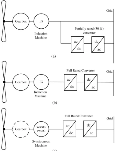
Figure1.2(a) shows a single-line diagram of the most common type of variable-speed wind turbine system (WTS) [9]. This configuration is made up of a variable-speed wind turbine connected to a doubly-fed induction generator (DFIG). The stator of the DFIG is directly connected to the grid while the rotor is connected to the grid via a partial-scale power converter which is typically rated at 20% - 30% of the generator power. The power converter is responsible for smooth grid connection and the variable speed range is ± 30% around the synchronous speed. Figures 1.2(b) and (c) show two variations based on the WTS showed in (a) but instead of a partial-scale power converter, makes use of a full-scale power converter. The generator can be either a wound-rotor synchronous generator (WRSG), a permanent magnet synchronous generator (PMSG) or an induction machine as used in (a). This concept has full control over the speed range from 0 to 100% of synchronous speed [9]. However, this concept provides higher losses when compared to (a) as all the power generated flows through the power converter.

1.2.3

Non-Conventional Wind Generator Concepts

Large wind turbines typically rotate at 30 - 50 revolutions per minute (rpm). The generator, either induction or synchronous, is required to rotate at speeds of 1000 - 1500 rpm in order to obtain the frequency needed for grid synchronization. This speed increase is achieved through the use of a gearbox. However, the inclusion of a gearbox incurs additional cost, weight and inefficiencies to the drivetrain.

Direct connection of the generator to the wind turbine (without a gearbox) would require the generator to have a large number of poles as described by (1.1) in order to produce the frequency required for grid connection (50 Hz or 60 Hz) while rotating at the relatively low speeds of 30 - 50 rpm, where P andN refer to the number of poles and rotational speed (in rpm) respectively.

F requency, f= P

2 ×

N

60 (1.1)

Permanent magnet synchronous generators (PMSG) are ideal for use in small-scale wind turbine applications. PMSG are synchronous machines where the rotor windings are replaced with permanent magnets. As a result, no external excitation is required so losses pertaining to rotor winding excitation are eliminated which allows for a higher power density at a small size. The permanent magnets allows for a smaller pole pitch which can yield a cost-effective design [10]. The small pole pitch also allows the PMSG to operate at lower speeds which either eliminates the need for a gearbox or allows for a single stage, low transfer ratio gears to provide for a more compact design.

However, synchronous generators (SG) exhibit oscillatory behaviour during load changes due to the limited amount of mechanical damping in the drivetrain and as a result, SG aren’t suited for direct-grid connection. It is common practice in industry to make use of damper windings but the small pole pitch required for wind turbine generator designs precludes the use of damper windings and as a result, damper windings aren’t considered suitable for wind energy applications involving PMSG.

IG Grid Gearbox Induction Machine Grid Gearbox Synchronous Machine WRSG/ PMSG (b) IG Grid Gearbox Induction Machine (c) (a)

Full Rated Converter Partially rated (30 %)

converter

Full Rated Converter

ac dc ac dc ac dc ac dc ac dc ac dc

Figure 1.2: Most common wind turbine drive-train layouts currently in use with (a) the variable speed doubly-fed induction generator (DFIG) with gearbox and partially rated converter,(b) the variable-speed doubly-fed induction generator (DFIG) with gearbox and full rated converter, (c) direct-drive wound rotor synchronous generator (WRSG) or permanent magnet synchronous generator (PMSG) and full rated power electronic converter. The gearbox is optional in (c).

Further attempts to provide a form of damping to the drivetrain have been made in literature. Figure

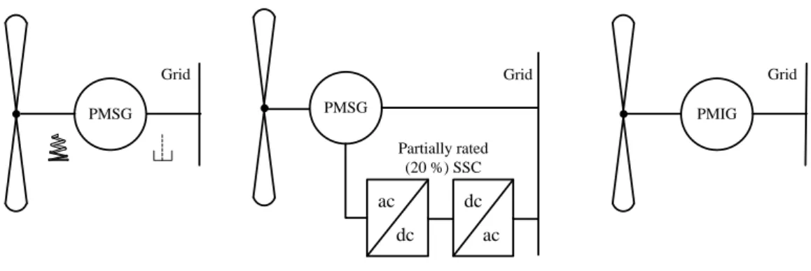
1.3(a) shows a spring and mechanical damper system proposed in [11] in which the stator is mounted on an additional bearing arrangement and is connected to the nacelle structure by means of the spring damper configuration. In [12], a small series partially rated converter (20% of rated power) is placed in the star point of the generator as shown in Figure 1.3(b). The series converter provides the damping required during input power or grid disturbances.

Another type of generator, the permanent magnet induction generator (PMIG), evaluated in [13] for direct-grid connection is shown in Figure 1.3(c). The PMIG consists of a conventional 3-phase stator winding, however, the rotor consists of two sections: an outer squirrel-cage rotor and an inner permanent magnet (PM) rotor. The outer rotor is connected to the wind turbine shaft while the PM rotor is allowed to rotate freely against the shaft. The PMIG operates by allowing the squirrel-cage rotor to be driven by an external force, the PM rotor rotates with this rotor at a slightly slower speed where the difference in speed is referred to as slip. It is this ’slip’ which provides a form of damping against torque pulsations. Once the squirrel cage rotor rotates at a speed greater than synchronous speed, the rotating PMs would induce a voltage in the stator with a frequency matching that of the grid’s voltage and synchronization can thus occur [13].

1.2.4

Slip-Synchronous Permanent Generator Concept

Figure 1.4 shows a wind turbine concept known as the slip-synchronous permanent magnet generator (SS-PMG), developed in [14], the topology is based on the PMIG concept discussed in the previous section. The SS-PMG consists of two integrated generating units: a slip permanent magnet generator (S-PMG) where the short-circuited rotor is directly mounted to the turbine and a PMSG unit of which the stator terminals are connected directly to the grid. The two machines are mechanically linked via a common, free rotating permanent magnet rotor with separate sets of magnets for each of the generating units [15]. The S-PMG operates in a manner similar to that of an induction machine. The short-circuited

PMSG Grid (a) PMSG Grid Partially rated (20 %) SSC (b) PMIG Grid (c) ac dc ac dc

Figure 1.3: Attempts to provide damping to a drivetrain including a PMSG with, (a) a spring and mechanical damper being used, (b) a PMSG with a partially rated star point converter and, (c) A direct-grid connected permanent magnet induction generator.

cage rotor rotates at a speed relative to that of the common PM rotor, where the difference in speed is again referred to as slip speed. The common PM rotor transfers mechanical power from the S-PMG to the PMSG unit which in turn generates electrical power. With the turbine directly connected to the short-circuited rotor which is intern magnetically connected to the common PM rotor which itself is magnetically connected to the PMSG stator, there is no physical connection between the wind turbine and the grid connected PMSG. As a result, the S-PMG stage provides a form of damping in the drivetrain against sudden wind disturbances which allows the SS-PMG to be directly grid connected, without the need for a power converter [14].

Grid

Slip Rotor

Permanent

Magnets

Stator

Common PM

Rotor

Figure 1.4: SS-PMG wind turbine drivetrain.

1.2.5

A Drivetrain Based off of The SS-PMG

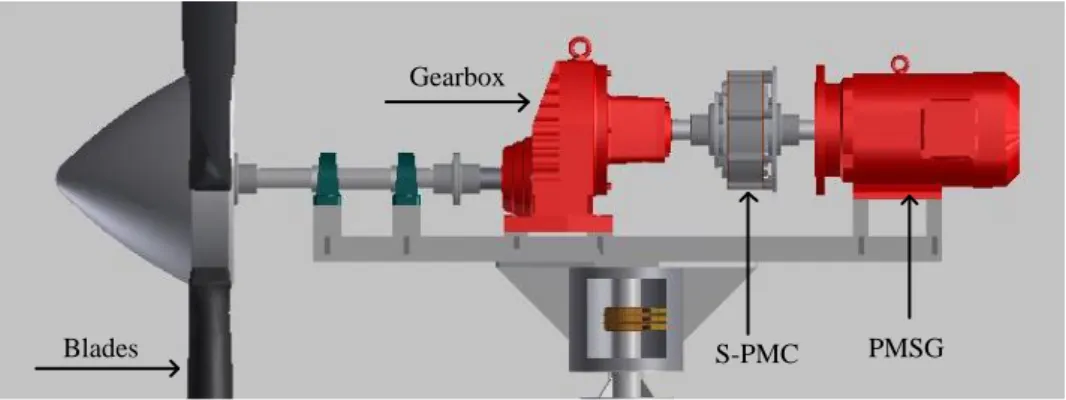
Figure1.5shows a new wind turbine drivetrain (based on the SS-PMG concept) proposed and developed in [16]. In this drivetrain, the SS-PMG is separated into two distinct machines: with one being a S-PMG (which is referred to as a slip permanent magnetic coupling (S-PMC) or ”slip coupler” in [16]) as previously described and the other being a conventional PMSG. The S-PMC is connected between the gearbox and the PMSG shown in Figure1.5. The S-PMC, shown in Figure1.6, consists of two rotating sections: the short-circuited rotor, (the inner section containing the windings), and an outer PM rotor. The drivetrain also includes a gearbox in order to provide greater flexibility with regards to speed selection.

Grid Short-Circuited Wound Rotor PM Rotor PMSG Gearbox

Figure 1.5: A wind turbine drivetrain concept based on the SS-PMG where the SS-PMG is separated into two distinct machines; with one being a S-PMC and the other a conventional PMSG.

Figure 1.6: CAD representation of the S-PMC assembly [17].

1.3

Generator Speed Control

In grid connected wind turbine systems (WTS), in the events leading to grid connection or in the event of a grid outage, the wind turbine rotor will continue to accelerate due to torque produced as a result of the wind. As a result, the international standards and certification rules require that two independent braking systems be used for large wind turbine systems and at least one braking system be used for smaller WTS. It is common practice to provide an aerodynamic braking system on the low-speed shaft and a mechanical brake on the high-speed shaft [18]. This section provides a brief overview of the various methods used to control the speed of wind turbines.

1.3.1

Power in the Wind

Equation1.2describes the power available in the wind,Pw, which can be defined as the amount of kinetic energy passing through a given area over time [19].

Pw=

1 2ρAυ

3_{, (1.2)}

whereρrepresents the air density in measured in (kg/m3),Ais the swept area of the wind turbine andυ is the speed if the wind (in m/s). However, the blades of a wind turbine cannot extract all of the energy in the wind and hence a term called the coefficient of wind power, Cp, is defined as the fraction of the wind power extracted by the wind turbine blades. Thus, the mechanical power, Pm, extracted from the wind by the turbine blades can be described as

Pm=

1 2ρCpAυ

3_{. (1.3)}

It is clear from1.2and1.3that the power produced by a wind turbine is heavily influenced by the speed of the wind, and consequently, the rotational speed of the turbine.

1.3.2

Pitch Control

For pitch controlled WTS, the turbine’s electronic controller monitors the turbine’s output power several times per second. When the turbine’s power output becomes too high, the electronic controller signals

the blade pitch mechanism to turn the rotor blades slightly out of the wind which reduces the overall lift required to rotate the turbine rotor. Conversely, the blades are turned back into the wind whenever the wind drops to levels which allow safe power production.

1.3.3

Stall Control

Stall controlled wind turbines have their rotor blades bolted to the turbine hub at a fixed angle. However, the blades are designed to ensure that the moment the wind speed becomes too high, the geometry of the blades creates turbulence on the side of the blade not facing the wind. This turbulence, or stall, prevents the lifting force of the rotor blade from acting on the rotor which limits the power produced by the turbine. The advantage of using stall control is that it avoids the use of moving parts and a complex control system. However, successful implementation of stall control requires complex aerodynamic design challenges relating to the dynamics of the whole wind turbine.

1.3.4

Active Stall Control

A common concept for larger wind turbines is to use what is known as active stall-regulation. Active stall machines resemble pitch controlled machines in the sense that they too have pitchable blades. However, the difference between active stall and pitch controlled machines is that if the generator is about to be overloaded, the active stall machine will pitch the blades in the opposite direction of that from what pitch controlled machined does. This is done to in order to force the blades into a deeper stall, thus wasting the excess energy in the wind. The advantage of active stall over normal passive stall controlled wind turbines is that the wind turbine can operate at near rated power at all high wind speeds.

1.3.5

Yaw Control

The yaw of a turbine refers to the angle between the incoming wind vector and the rotational axis of the turbine. To ensure maximum power extraction, the turbine should always be aligned with the wind, i.e., a yaw angle of zero. Wind turbines that make use of yaw control have what is known as a yaw drive which is responsible for directing the turbine into the wind based off signals received from various sensors located on the wind turbine nacelle. Furthermore, the yaw drive can also steer the turbine out of excessive incoming winds.

1.3.6

Electro-Mechanical Braking

One way to slow down and halt a wind turbine rotor involves converting the rotational kinetic energy into heat. This type of braking system is referred to as a mechanical disk brake. Disk brakes are mounted on the shaft (either the low-speed shaft, high-speed shaft or both) and slow the turbine down by providing breaking torque in the form of friction. Disk brakes provide overspeed control, parking and emergency braking of wind turbines. However, one disadvantage of using a disk brake (in large wind turbines) is the inherent operating delay which can be as long as 10 seconds [20]. During this time, the rising rotor speed could accelerate to dangerous levels which could damage the wind turbine.

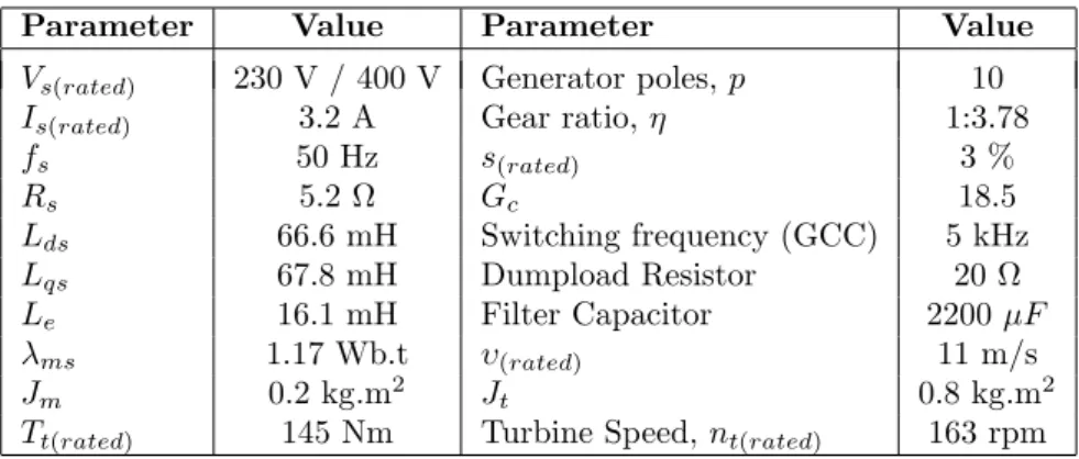
Another braking system proposed in [10] and shown in Figure 1.7(a) is known as electrodynamic braking in which counter-torque produced by the generator itself is used to brake the turbine. This system involves connecting a resistive bank to the terminals of the generator. The resistors are connected in parallel and with the appropriate switches, the value of resistance and hence the load on the generator can be varied to control the speed of the rotor.

A variation to the resistor bank braking method is proposed in [21] and shown in Figure1.7(b) is used to provide speed control for a SS-PMG in which the resistor bank is replaced by a thyristor pack which is able to achieve variable braking torque with a single resistor. This is achieved by varying the thyristor firing angle. In this way, the generator counter-torque can continuously varied to respond to changing conditions without the need for multiple resistors [21].

Grid _Grid

(a) (b)

Figure 1.7: Line diagram of, (a) the resistive bank based speed control strategy and (b) the thyristor based single resistor strategy with optional resistor stages shown with dotted lines [21].

1.4

Generator Synchronization Conditions

Figure 1.8 shows a generator G1 supplying power to a load with a second generator, G2 about to be synchronized to the local network through contactorS1[22]. However, beforeG2can be connected to the network, each of its three phases must have exactly the same voltage magnitude and phase angle prior to S1 closing. Additionally,G1’s voltage frequency should be equal to that of G2. IfS1is closed at any arbitrary moment where the voltages and frequency ofG2 aren’t exactly the same in each conductor as those of G1, both generators are liable to be severely damaged by the large inrush currents and power transients that will occur before the generators stabilize at a common frequency [22]. Furthermore, these inrush currents and power transients could result in a loss of power to the load. Table 1.1provides the general guidelines for synchronizing generators to existing power systems.

From Table 1.1, prior to synchronization, the difference in frequency, 4f, rms phase voltage 4V, and, voltage-phase angle,4φbetween the oncoming generator and the connected generator must be less than a predetermined limit depending on the size of the generator.

G

G

Load

S1

Figure 1.8: An oncoming generator (G2) being connected to a power system [22].

Table 1.1: Parameter limits for synchronisation with the Eskom distribution network [23].

Embedded Generator Rating [kVA] Maximum Frequency Difference [Hz] Maximum Voltage Difference [%] Maximum Phase Angle Difference [◦] 0 ≤S <500 0.3 10 20 500 ≤S <1500 0.2 5 15 S≥1500 0.1 3 10

1.5

Turbine Torque Pulsations

The power produced by wind turbines under continuous operation often include periodic fluctuations at n times the rotational frequency of the blades (ft) or nft where n is the number of blades [24, 25]. The most prominent of these frequency fluctuations are due to two phenomena known as wind sheer and tower shadow. Wind shear refers to the variability of wind speed with respect to height [24], in other words, the wind speed at the tip of a turbine blade (when the tip of the blade is facing upwards) will be greater than the wind speed experienced at the blade’s hub-point connection. Tower shadow refers to the disruption and redirection of airflow as a result of the turbine tower. Furthermore, each time a turbine blade passes in front of the tower, the disrupted airflow causes a fluctuation in the mechanical torque produced by the blade. This fluctuation in torque is then transferred to the generator which results in a small dip in output power [26]. The tower shadow effect is known to produce the most significant of turbine torque pulsations when compared to wind sheer [24,25,26]. Thenft frequencies are dependent on the rotational speed of the turbine and as a result, the generator will experience periodic dips in mechanical torque in the frequency range of 0.5 - 10 Hz [26]. This low frequency range tends to cause fluctuations in system rms voltage (known as voltage flicker) at the point of common connection (PCC) -where the wind turbine connects to the grid- which negatively effects the power quality supplied to the grid [26]. The tower shadow effect is known to be most prominent in downwind turbines due to the turbine tower being directly in the path of airflow prior to hitting blades. This in contrast to upwind turbines where the airflow strikes the bladesbefore it hits the tower.

1.6

Statement of the Problem

Permanent magnet synchronous generators (PMSG) have shown to be an ideal solution for small-scale wind turbine applications. However, PMSG cannot be direct-grid connected as a result of a lack of damping present in conventional drivetrains. Attempts have been made in literature to provide damping to the drivetrain with a partial or full rated power converter being the favoured option in industry. However, full scale power converters (or even partial scale converters) impose penalties which include cost, reliability and efficiency.

The SS-PMG or the drivetrain based on the SS-PMG concept are wind turbine systems which can be connected to the grid without the need for a power converter. However, without a power converter providing smooth grid connection, a new means to synchronize slip-synchronous wind turbine systems (SS-WTS) to the grid is needed.

The wind turbine drivetrain from Figure 1.5 is to be used in a downwind configuration and is to be connected to an electrical network without the use of a power converter. That is to say, before grid connection, the new synchronization system would need to be able to allow the downwind turbine drivetrain to accelerate from rest to synchronous speed and then maintain the generators speed at synchronous speed prior to grid connection. Furthermore, the synchronization system would be required to disconnect the downwind turbine drivetrain from the grid in the event where the downwind turbine ceases to produce power and instead, starts to draw power from the grid.

Additionally, once grid connected, the downwind turbine’s dynamic stability remains a concern. As stated in previous sections, PMSG exhibit oscillatory behaviour in the presence of load changes. Furthermore, with the wind turbine being in a downwind configuration, the effects of wind sheer and tower shadow become more prevalent. It remains unknown whether or not a downwind turbine, making use of a slip coupler (S-PMC), can provide sufficient damping to the drivetrain in order to mitigate the oscillatory behaviour known to occur in direct grid connected PMSG-based wind turbine systems.

1.7

Objective of Study

The drivetrain shown in Figure 1.5 is to be used in a downwind configuration. However, before the downwind wind turbine can be considered for real world application, a speed controller which is to be used in conjunction with a grid connection controller (GCC) needs to be developed and tested which would allow the downwind turbine to synchronize with and connect to the grid. Consequently, the speed controller and GCC should be able to:

• Allow the wind turbine drivetrain to accelerate from rest until it reaches synchronous speed.

• Once the wind turbine has reached synchronous speed, the speed controller must be able to maintain the generator’s speed at synchronous speed.

• Once synchronous speed as been established and maintained, the GCC will monitor and wait for the generator’s voltage magnitude, frequency and phase to match that of the grid’s.

• After all the necessary synchronization requirements have been met, the GCC will then connect the wind turbine to the grid.

The objectives are thus to determine a transfer function model of the downwind turbine drivetrain from which a speed controller can be designed and tested. The speed controller must be able to control and maintain the downwind turbine drivetrain speed (from rest) at synchronous speed regardless of the wind speed.

A further objective was, once the downwind turbine is connected to the grid, how well does it perform against turbulent winds, especially those pertaining to the 3ft frequency which is known to cause substantial torque pulsations in downwind turbines.

The final objective was to evaluate the performance of the downwind turbine in real-world applications. The downwind turbine is to be tested at Stellenbosch’s Mariendahl wind turbine testing facility.

1.8

Significance of the Study

The significance of the study is that it contributes to the development and understanding of direct-grid connected slip-synchronous wind turbine systems (SS-WTS). The slip-synchronous permanent magnet generator (SS-PMG), described in Section 1.2, has shown to be a suitable wind turbine system for direct-grid connection application. However the lack of a gearbox limits the SS-PMG to relatively low speeds which in turn forces the machine to be large and bulky. Furthermore, the design of the SS-PMG concept imposes a complexity in the design of the drivetrain as it requires two generating units which are magnetically coupled by a common PM rotor.

For these reasons, the separation of the two generating units as well as the inclusion of a gearbox allows for a greater speed selection which in turn allows for a physically smaller generator and a more compact wind turbine system. However, unlike the SS-PMG, the newly proposed and developed drivetrain of Figure 1.5has yet to be tested in a laboratory or in the field. This fact furthers the significance of this study as the results may be utilized to develop and improve the overall design of SS-WTS as well as the systems used to synchronize these SS-WTS to utility grids without the need for power converters. The overall goal of the study is to further the knowledge of new, novel wind turbine systems.

1.9

Thesis Structure

The mathematical modelling of the downwind turbine is addressed in Chapter 2. Furthermore, the mathematical model is then used to develop a simulation model of the downwind drivetrain in MATLAB/Simulink. The design of the speed controller is handled in Chapter 3. Chapter 4 deals with the dynamic performance of the grid connected wind turbine model under turbulent wind/torque conditions. Chapter 5 attempts to verify the MATLAB/Simulink Model of the downwind drivetrain on a testbench in the laboratory. Chapter 6 deals with the real-world performance of the downwind turbine where field test results obtained from Stellenbosch’s wind turbine testing facility will be presented.

Chapter 2

Modelling

This chapter develops a dynamic simulation model for the downwind turbine drivetrain shown in Figure

2.1. The drivetrain model will be implemented in MATLAB/Simulink in order to evaluate the downwind drivetrain’s performance under varying simulated conditions. The dq-reference frame will be used to model the permanent magnet synchronous generator (PMSG) whereas the slip-magnetic coupling (S-PMC) will be modelled based off of it’s linear slip versus torque relationship. The wind turbine is modelled using a function generator developed from the turbine’s torque-speed curves and the gearbox is treated as a one-lump mass model for simplicity. Finally, a brief description of the grid connection controller (GCC) and it’s functionality is provided at the end of the chapter.

Blades

Gearbox

S-PMC PMSG

Figure 2.1: A CAD representation of the downwind turbine drivetrain.

2.1

PMSG

The permanent magnet synchronous generator (PMSG) was designed and constructed in [27]. Figure

2.2 (a) and (b) show the respective permanent magnet (PM) rotor and the wound stator of the PMSG. The PMSG consists of a 10/12 pole/slot combination with permanent magnets on the rotor providing the magnetic field. The stator is made up of double-layer, non-overlap copper windings with a fill factor of 40%. The PMSG is directly grid connected via a grid connection controller (GCC) and operates at a synchronous speed of 600 revolutions per minute (rpm). Furthermore, the rated power of the PMSG is 2200 W and its rated torque is 36 Nm.

The dq-equivalent circuits of the PMSG are shown in Figure 2.3 and the consequent dq-dynamic equations are given by

vqs = −Rsiqs−Lqs diqs dt −ωeLdsids+ωeλms, vds = −Rsids−Lds dids dt +ωeLqsiqs, (2.1)

where ωe represents the electrical speed in radians per second (rad/s). The stator winding resistance is given as Rs and the flux-linkage due to the permanent magnets is given by λms. The PMSG dq-inductances are given byLds andLqs and are determined by

(a) (b)

Figure 2.2: Figure showing the constructed PMSG rotor (a) and wound stator (b) [27].

s

R

R

v

v

L i



e



 

L i



i

i

L

L

Figure 2.3: The dynamicdq-equivalent circuits of the PMSG.

Lds= λd−λms −Id +Le; Lqs = λq −Iq +Le, (2.2)

whereLerepresents the end-winding inductance. Finally, the torque generated by the PMSG is given by

τs= 3

4p[(Lqs−Lds)idsiqs+λmsiqs]. (2.3)

where prepresents the number of generator poles.

2.2

S-PMC

The slip-magnetic coupling (S-PMC) used in the drivetrain was designed and constructed in [16]. The S-PMC consists of two rotating sections which are shown in Figure2.4. The first section, Figure2.4(a), consists of a short-circuited rotor (the inner section containing the windings) whereas the second section, Figure 2.4(b), consists of a PM rotor (the outer section, lined on the inside with PMs). The magnetic coupling allows for the transfer of torque between the gearbox and the PMSG and acts as a filter for torque transients with the aim of improving the quality of the torque transmitted to the PMSG. The S-PMC consists of a 28/30 pole/slot combination, with all 30 non-overlap coils short-circuited and has an efficiency of 97% [16]. Furthermore, like an induction machine, the S-PMC operates under slip conditions where the slip is proportional to the amount of torque being transferred. The formal definition for slip speed is defined as

nslip=nsync−nm (2.4)

wherenslipis the slip speed,nsyncis the synchronous speed andnmis the mechanical shaft speed (all in rpm). The termslip is the relative speed expressed on a per-unit basis [22] and is defined as

s= nslip nsync

(×100%) = nsync−nm nsync

(×100%). (2.5)

If equations (2.4) and (2.5) are expressed in terms of angular velocityω, then for the S-PMC,

ωsl =ωm−ωs= (

ωm−ωs ωm

(a) (b)

Figure 2.4: Figure showing the constructed S-PMC short-circuited rotor (a) and the PM rotor (b) [16].

whereωsl is the slip speed, ωm=ωe×2_p is the rotor speed (on the high-speed side of the gearbox) andωsis the PMSG rotor speed or if grid connected, synchronous speed, all in rad/s.

Figure2.5(a) [16] shows the linear relationship between slip and the output torque produced by the S-PMC. The output torque,τr, is described by

τr=Gc×ωm×s, (2.7)

where the S-PMC gain (Gc) is given by

Gc= τr s×ωm

(2.8) and shown in Figure2.5(b).

(b) 0 0.2 0.4 0.6 0.8 1 1.2 1.4 1.6 1.8 0 0.5 1 1.5 2 2.5 3 3.5 4 4.5 5 5.5 T or q u e ( p .u .) Slip (%) (a)

G

τ

ω

Figure 2.5: S-PMC modelling with (a) the linear relationship between slip and torque for slip values between (0 - 5%)[16] and (b) the S-PMC gain block model.

2.3

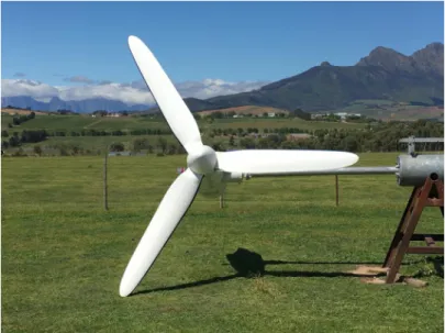
Turbine Blade Model

Figure2.6shows the three blades of the downwind turbine fitted to the nacelle. Wind turbine blade sets are characterised by their wind power coefficient (Cp) versus Tip-Speed-Ratio (TSR) curve where the TSR is defined as

T SR= ωR

υ , (2.9)

whereω is the turbine angular velocity (in rad/s),Ris the length of one of the blades andυ is the wind speed (in m/s). TheCpversus TSR curve for the 1.9 m blades used for the downwind turbine is shown in Figure2.7. Figure2.8(a) shows the wind turbine’s power-speed curves and Figure2.8(b) shows a function

Figure 2.6: Downwind turbine blades.

generator representation model which provides the aerodynamic torque produced by the turbine as an output based off of the wind turbine’s power-speed curves with wind speed, v and turbine rotational speed, ωtas inputs to the function generator.

0 0.05 0.1 0.15 0.2 0.25 0.3 0.35 0.4 0.45 0 1 2 3 4 5 6 7 8 9 10 11 12 13 14 Wi nd P ow er C oef fi ci ent -Cp Tip-Speed-Ratio

Figure 2.7: Wind power coefficient versus tip-speed-ratio curve for the 1.9 m blade set used for the downwind turbine [16].

Function

Generator

v

ωt

τt

Figure 2.8: Wind turbine power versus turbine speed curves (a)[16] and equivalent simulation block model (b).

2.4

Gearbox

The drivetrain gearbox is anSEW Eurodrivewith a gear ratio of 1:3.78, a maximum torque rating of 305 Nm, and a power rating of 5 kW. It is a single stage, helical gear unit which is used as an up-speed gearbox to increase the drivetrains rotational speed by a factor of 3.78. Tests conducted in [16] determined the gearbox efficiency and it was found to be 96-97% at a load of 132 Nm. However, it should be noted that this efficiency could only be reached once the gearbox is brought to the rated operating temperature by running the gearbox under rated load for 1.5 hours [16].

For simplicity, the gearbox is modelled as a gain-block where its magnitude is that of the gear ratio, 1 : 3.78, as its purpose in the simulation model is to reduce the turbine torqueτtby a factor of 3.78. As a result the dynamics of the turbine and slip-rotor are expressed as

τt0−τ_r=J_t

dωt

dt , (2.10)

while the dynamics of the PM rotor section and the PMSG are given by

τm=τr−τs=Jm dωs

dt , (2.11)

where τt0 is the torque generated by the turbine reduced by a factor of 3.78, τ_r is the torque generated

by the S-PMC and τm is the resultant torque acting on the PMSG rotor. The respective inertias of the turbine (plus the S-PMC’s short-circuited rotor) and the PMSG (plus the S-PMC’s PM rotor) are represented by JtandJm.

2.5

Grid Connection Controller

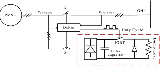
Figure 2.9 shows a simplified model of the grid connection controller (GCC). The GCC is responsible for controlling the speed of the downwind turbine prior to grid connection as well as synchronizing and connecting the downwind turbine to the grid. The GCC achieves this by comparing the frequency of both the generator and the grid through the method of counting the zero crossings of their respective terminal voltages over a specified time period. The error in frequency is then fed into a digital PI-controller which adjusts the duty cycle of a dumpload chopper circuit which regulates the effective load at the terminals of the generator, which in turn controls the speed of the wind turbine. Once the frequency of the generator matches that of the grid, the GCC waits for the respective voltage phase angles of the generator and grid to align before closing S1 (normally open) and opening S2 (normally closed) and connecting the generator to the grid.

Additionally, the GCC will disconnect the grid-connected wind turbine (by openingS1and connecting the dumpload to the stator terminals) in the event where: the generator no longer produces power, the power produced by the wind turbine exceeds operational conditions, or in any event where the grid code is violated. F i l t e r C a p a c i t o r D u m p L o a d D s P i c G r i d I G B T S1 P M S G va b c ( g e n ) va b c ( g r i d ) D u t y C y c l e S2

Dumpload Chopper Circuit

2.6

Downwind Turbine Simulation Parameters

Table2.1provides the relevant parameters used in the chapters and sections that follow. Table 2.1: Downwind turbine simulation parameters.

Parameter Value Parameter Value

Vs(rated) 230 V / 400 V Generator poles,p 10

Is(rated) 3.2 A Gear ratio,η 1:3.78

fs 50 Hz s(rated) 3 % Rs 5.2 Ω Gc 18.5 Lds 66.6 mH Switching frequency (GCC) 5 kHz Lqs 67.8 mH Dumpload Resistor 20 Ω Le 16.1 mH Filter Capacitor 2200µF λms 1.17 Wb.t υ(rated) 11 m/s Jm 0.2 kg.m2 Jt 0.8 kg.m2

Tt(rated) 145 Nm Turbine Speed,nt(rated) 163 rpm

The turbine inertia referred to in Table 2.1 represents the estimated turbine inertia transferred to the generator side of the simulation according toJt=JT/η2 whereJT is the actual turbine inertia andη is the gear ratio of the gearbox.

2.7

Model Implementation

From the mathematical equations in the previous sections a complete simulation model of the downwind turbine is obtained and shown in Figure 2.10. The input to the simulation model is wind speed, vwind whereas the outputs are the PMSG’s terminal 3-phase voltages va, vb and, vc. The simulation model is implemented in MATLAB/Simulink in order to evaluate the drivetrain’s performance under various simulation conditions.

v





ω

ω

ω

-+

ω

ω

τ

τ’

+

-τ

s

J

1

v

v

v

τ

Chapter 3

PI Speed Controller Design

In this chapter, the necessary proportional (P) and integral (I) components of a PI-controller are developed. The PI-controller is implemented in MATLAB/Simulink in conjunction with the downwind turbine model developed in Chapter 2. A closed-loop block diagram model of the downwind turbine drivetrain, the PI-controller, and the GCC is then used to evaluate the the PI-controller’s ability to maintain the downwind turbine’s speed at synchronous speed for any given wind speed.

3.1

Downwind Drivetrain System Identification

One of the first steps in designing a control system is to identify and understand the dynamic performance of theprocesswhich is to be controlled [28]. This can be done theoretically where the process is modelled using mathematical equations or by using experimental data to generate a model for the process. In this section, the downwind turbine drivetrain model is treated as an ”unknown” process for which a simplified first-order plus dead time (FOPDT) is developed.

3.1.1

Dynamic Step-Test of the Downwind Turbine Drivetrain Process

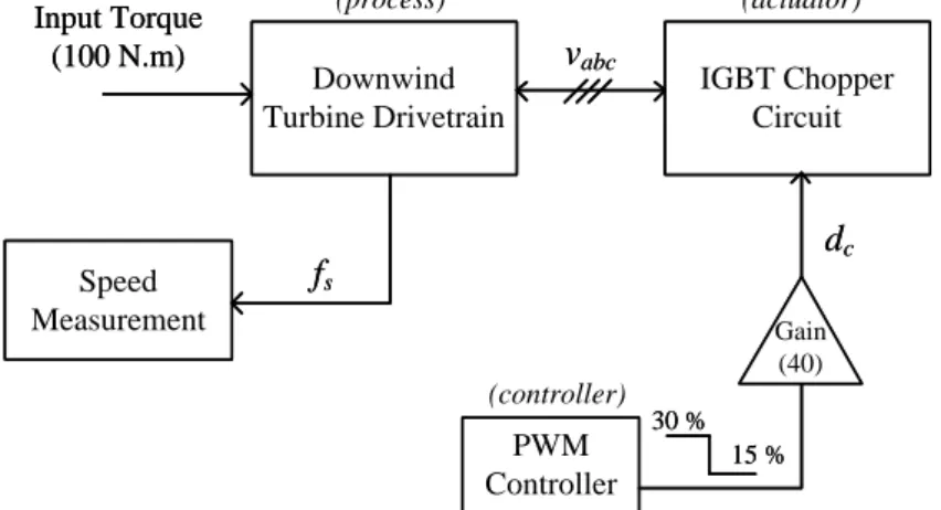
In the presence of consistent wind, wind turbines will accelerate indefinitely if not connected to a load or braking mechanism. This kind of behaviour is referred to as non-self-regulating or integrating. In contrast,self-regulating processes are those which naturally settle at some steady-state value for a given input. The downwind drivetrain, from Figure 2.10, is anon-self-regulating process with regards to its input (wind speed) and its output (frequency). However, by connecting a pulse-width modulated (PWM) controlled dumpload chopper circuit to the terminals of the generator, for any given wind speed (referred to as input torque from here on) and for a predetermined duty cycle, the downwind drivetrain’s output will settle at some steady-state speed and consequently behave as aself-regulating system.

Figure3.1shows a block diagram representation of a dynamic step-test performed on the downwind turbine drivetrain and Figure 3.2 shows the result of the dynamic step-test. The dynamic step-test involved providing the simulated drivetrain and chopper circuit model with an initial disturbance, in this case a constant input torque signal of 100 Nm, while the duty cycle to the chopper circuit is initially held at a constant level of 30%. Due to the input torque, the drivetrain will initially accelerate before settling at a steady-state speed as a result of the counter-torque produced by the generator due to the effective load at its stator terminals. After the drivetrain’s speed has settled at a steady-state level, the duty cycle is then stepped down to 15% (with no change to the input torque disturbance signal) to allow the drivetrain’s speed to accelerate and once again settle at a new steady-state level. From this dynamic step-test, a FOPDT model for the downwind turbine drivetrain and dumpload chopper circuit can be developed which describes the relationship between the duty cycle, (dc), and speed (fs) for a constant input torque.

3.1.2

First-Order Plus Dead Time Model

A first-order plus dead time dead time transfer function model is, in general, described by

G(s) = kpe −τds

τps+ 1

, (3.1)

where G(s) represents the transfer function of the identified process. The process gain (kp) is defined as the change in process output (4fs) over the change in controller output (4dc). The process time constant (τp) is defined as the time taken before the process output reaches 63% of its final value and

Downwind Turbine Drivetrain IGBT Chopper Circuit PWM Controller

v

d

f

v

d

f

Figure 3.1: Block diagram model of the dynamic step-test performed on the downwind turbine drivetrain.

Duty Cycle (%) Speed (Hz) 0 5 10 15 20 25 30 35 40 45 50 0 5 10 15 20 25 30 35 40 45 50 0 2 4 6 8 10 12 14 16 18 20 22 24 Time (s)

Duty Cycle (%) Speed (Hz) FOPDT (Hz)

Δdc

Δfs

Figure 3.2: Simulated dynamic step-test results for a change in duty cycle (dc) from 30% to 15 % for a constant input torque of 100 Nm, and a dumpload resistor value of 20 Ω.

the process dead time (τd) is defined as the delay in time before the process responds to the change in controller output.

From Figure3.2over the time ranget≥10 seconds,

• kp=|4₄f_ds c|=| (47−25) (15−30)·40|= 0.03667 • τp'2 seconds and, • τd'0.02 seconds.

The FOPDT transfer function model for the downwind turbine drivetrain and IGBT chopper circuit is thus

G(s) = 0.03667e −0.02s

2s+ 1 , (3.2)

where the accuracy of the FOPDT transfer function model is shown in Figure3.2.

3.1.3

Discussion

The downwind turbine drivetrain simulation model behaves as a self-regulating process for a constant torque input and set duty cycle. That is to say, in the presence of a torque input, the drivetrain will accelerate before settling at a steady-state speed as a result of the set duty cycle. However, the downwind drivetrain can also be seen as a near-integrating process. A near-integrating process is defined as a self-regulating process whose process time constant is much larger than its process dead-time. For this

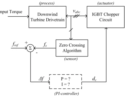
reason, the downwind turbine drivetrain can be viewed as a near-integrating process. Furthermore, the downwind drivetrain exhibits further integrating characteristics in the sense that the dynamic step-test will yield different process values (kp and τp) for different input torque and duty cycle combinations. This is problematic when considering that most PI-control algorithms are designed off of the values of kp and τp. Consequently, a suitably robust PI-control algorithm is needed in order to implement speed control regardless of changing process dynamics. Furthermore, the PI-controller will replace the manually controlled PWM-controller shown in Figure3.1 and will automatically control the duty cycle input to the chopper circuit based on the difference in frequency between the downwind drivetrain and a predetermined reference frequency. Figure 3.3 shows the resulting block diagram required to provide automatic, closed-loop speed control.

Downwind Turbine Drivetrain IGBT Chopper Circuit

v

f

+

f

-Δf

d

Figure 3.3: Block diagram model of the required PI-controlled speed controller.

3.2

PI Tuning

There are more than 400 PI and PID tuning methods from which to develop a controller [29] with the most common of those being:

1. Ziegler-Nichols Tuning, 2. Cohen-Coon Tuning, 3. Lambda Tuning and,

4. Internal Model Control (IMC).

The Ziegler-Nichols tuning rules work well for processes whose time constant (τp) is at least two times as long as the process dead time (τd) whereas the Cohen-Coon tuning method works well for processes where the process time constant is greater than at least half of the process dead time [30]. As a result, the Cohen-Coon tuning method is suited to a wider variety of processes than the Ziegler-Nichols method [30]. Both the Ziegler-Nichols and Cohen-Coon tuning rules are based off of the Quarter Decay Ratio [28] otherwise known as Quarter Amplitude Damping [30] where the control objective is to eliminate any error between the set-point and process output as quickly as possible. However, the speed of the controller often results in the process output overshooting the set-point and oscillate around the set-point before reaching the set-point steady-state value [29].

Lambda and Internal model control (IMC) tuning offer an alternative to quarter amplitude tuning. Both Lambda and IMC tuning aim for a first-order plus dead time response to a change in set-point [29]. Furthermore, both Lambda and IMC tuning rules have the following advantages [30]:

• Lambda and IMC tuning rules are much less sensitive to any errors made when determining the process dead time through dynamic step-tests.

• The tuning is very robust, in other words, the control loop will remain stable even if the process dynamics/characteristics change from the ones used for tuning.

• The Lambda and IMC control loops absorbs a disturbance better, and passes less of it on to the rest of the process.

One of the drawbacks of Lambda and IMC tuning is that the controller’s integral time (Ti) is set equal to some multiple of the process time constant [30]. Consequently, if the process has a long time constant, the resulting lengthy integral time will result in a slow recovery time from disturbances. [30].

However, due to the flexibility towards changes in the dynamics of the process model as well as the robustness of the control loop that IMC and Lambda tuning methods provide makes them the ideal choice for developing the PI speed controller used by the GCC to control the speed of the downwind drivetrain.

3.2.1

Internal Model Control Tuning

The internal model control (IMC) tuning rules are based off of the values:

• kp - process gain,

• τp - process time constant,

• τd - process dead time,

which are determined from the results of the process’ dynamic step-test. The above listed parameters are used to determine the necessary proportional (P) and integral (I) parameters of a PI-controller. The controller gain, Kc, for a self-regulating process is calculated as [30]

Kc= 1 kp × τp (τd+τc) . (3.3)

However, the process gain of a self-regulating process whose process time constant is much larger than its dead time can be converted to an integrating process gainki by using [31],

ki= kp τp

. (3.4)

The parameter, τc, is referred to as the closed-loop time constant where a small value ofτc results in a faster control loop. Furthermore, it is suggested in [30] that the value ofτc be 1-to-3 times that ofτp. Using (3.3) with the values obtained from the downwind drivetrain dynamic step-test, the proportional P term is set equal to the controller gain and is subsequently determined by [30]:

P =Kc = 1 0.03667 × 2 (0.02 + 2) = 27.

If the downwind drivetrain is treated as a near-integrating process, the proportional term is calculated as

P =Kc = 1 ki × τp (τd+τc) = 1 0.018335× 2 (0.02 + 2) = 54, where ki is calculated as ki= kp τp =0.03667 2 = 0.018335.