On the Equivalence of Location Choice Models:
Conditional Logit, Nested Logit and Poisson
K
URT
S
CHMIDHEINY
M
ARIUS
B
RÜLHART
CES
IFO
W
ORKING
P
APER
N
O
.
2726
C
ATEGORY12:
E
MPIRICAL ANDT
HEORETICALM
ETHODSJ
ULY2009
An electronic version of the paper may be downloaded
• from the SSRN website: www.SSRN.com
• from the RePEc website: www.RePEc.org
CESifo
Working Paper No. 2726
On the Equivalence of Location Choice Models:
Conditional Logit, Nested Logit and Poisson
Abstract
It is well understood that the two most popular empirical models of location choice -
conditional logit and Poisson - return identical coefficient estimates when the regressors are
not individual specific. We show that these two models differ starkly in terms of their implied
predictions. The conditional logit model represents a zero-sum world, in which one region's
gain is the other regions' loss. In contrast, the Poisson model implies a positive-sum economy,
in which one region's gain is no other region's loss. We also show that all intermediate cases
can be represented as a nested logit model with a single outside option. The nested logit turns
out to be a linear combination of the conditional logit and Poisson models. Conditional logit
and Poisson elasticities mark the polar cases and can therefore serve as boundary values in
applied research.
JEL Code: C25, R30, H73.
Keywords: firm location, residential choice, conditional logit, nested logit, Poisson count
model.
Kurt Schmidheiny
Department of Economics
University Pompeu Fabra
Ramon Trias Fargas 25-27
Spain – 08005 Barcelona
[email protected]
Marius Brülhart
Department of Economics
School of HEC
University of Lausanne
Switzerland – 1015 Lausanne
[email protected]
July 14th, 2009
We are grateful to Paulo Guimaraes and his coauthors for allowing us to use their data set,
and to seminar participants at Pompeu Fabra and at the University of Barcelona for useful
comments. Financial support from the Spanish Ministry of Science and Innovation (Ramon y
Cajal and Consolider SEJ2007-64340), the Swiss National Science Foundation (grants
100012-113938 and PDFMP1-123133), and from the EU's Sixth Framework Program
(“Micro-Dyn” project) is gratefully acknowledged.
1
Introduction
Location choices by households and firms are of interest to economists for numerous reasons, ranging from the determinants of residential segregation patterns in cities to the design of national tax policy. Given the discrete nature of such choices, they are typically modelled by empirical researchers through McFadden’s (1974) conditional logit framework.1 The ap-peal of this approach lies in its formal link between the theoretical objective function of a representative location-seeking agent and the likelihood function of the empirical model.
Mostly out of a perception of greater computational ease, researchers have resorted to Poisson count estimation as an alternative approach to the conditional logit.2 Guimaraes, Figueiredo and Woodward (2003), henceforth GFW, have shown that, with purely location-specific locational determinants or with determinants that are location-specific to locations and to groups of agents, the conditional logit and Poisson estimators return identical parameter estimates. In this sense, the two estimators are equivalent, and the rigorous link to the theory offered by the conditional logit model therefore applies identically to the Poisson. This useful result has already been applied widely in the location choice literature.3
We show that the identical coefficient estimates resulting from the two estimation strate-gies in fact have fundamentally different economic implications. The conditional logit model implies that the aggregate number of agents is fixed and that differences across locations affect only the distribution of those agents across those locations. Hence, an additional agent at-tracted to locationjmeans one less agent among the other locations in the relevant set,i6=j. In the Poisson model, however, an additional agent attracted to location j has no impact on the number of agents in the remaining locations and thus raises the aggregate number of agents, summed across i and j, by one. Thus, the conditional logit model and the Poisson model can be viewed as polar cases, with the former representing zero-sum reallocations of firms or households across locations and the latter implying a positive-sum world.4
We also show that intermediate cases between these two extremes can be represented by a nested logit model featuring a generic outside option. This approach returns the same
1
For studies of firm location choices using the conditional logit approach, see, e.g., Carlton (1983), Head, Ries and Swenson (1995), Guimaraes, Figueiredo and Woodward (2000), Head and Mayer (2004), Crozet, Mayer and Mucchielli (2004), and Devereux, Griffith and Simpson (2007). For corresponding studies of household location chocies, see, e.g., Ellickson (1981), Quigley (1985), Nechyba and Strauss (1998), Schmidheiny (2006), and Bayer, Ferreira and McMillan (2007).
2
See, e.g., Papke (1991), Becker and Henderson (2000), List (2001), Guimaraes, Figueiredo and Woodward (2004), and Holl (2004), for studies of firms’ location choices; and Flowerdew and Aitkin (1982) and B¨ orsch-Supan (1990) for studies of individual migration choices.
3Recent studies invoking the GFW equivalence result include Duranton, Gobillon and Overman (2006), Br¨ulhart, Jametti and Schmidheiny (2007), Arzaghi and Henderson (2008), Davis and Henderson (2008), and Coeurdacier, De Santis and Aviat (2009).
4For recent research on the cross-region effects of region-specific policies aimed at attracting firms, see, e.g., Greenstone and Moretti (2003), Chirinko and Wilson (2008), and Wilson (2009).
parameter estimates as the two other estimators. The nested logit in fact can be written as a linear combination of the conditional logit and Poisson models, with a single “rivalness parameter” representing the closeness of the nested logit to the conditional logit (and thus the distance from the Poisson). Conditional logit and Poisson elasticities mark the polar cases and can therefore serve as boundary values in applied research.
The paper is structured as follows. In Section 2, we formally derive the commonalities and differences among the conditional logit, Poisson and nested logit models. Empirical implications and an illustration are presented in Section 3. Section 4 concludes.
2
The models
We denote agents with f = 1, ..., N and regions with j = 1, ..., J. For simplicity, we shall frame our discussion in terms of corporate location decisions, and therefore relate to f as “firms”.
Following GFW, we first assume the determinants of locational attractiveness to be purely region specific, such that they affect all firms symmetrically (case A). The K observable characteristics of each region are given by the (K×1) vectorxj. We then relax this assumption,
and allow locational attractiveness to be region-industry specific (case B).
The random variablenj represents the count of firms in regionj, whereasNj denotes the
number of firms actually observed in regionj. Analogously, the random variablenrepresents the total number of firms, whereasN denotes the observed total number of firms.
2.1 Case A: industry-invariant locational determinants
2.1.1 Conditional logit
Suppose that firm f’s profit in region j is determined by the linear model πf j = x0jβ+εf j,
whereβ is a (K×1) vector of coefficients. Then, the conditional logit model is defined by the assumption that the random termεf j is independent across f and j and follows an
extreme-value type 1 distribution. With this assumption, the probability that a given firm f chooses regionj rather than another region is given by
Pj|f =Pj = ex0jβ PJ i=1ex 0 iβ , (1) whereP
jPj|f = 1 for all f. Since locational characteristicsxj are assumed here to affect all
firms symmetrically, this probability also represents the share of firms that will choose region j.
The parameterβcan be estimated by maximum likelihood. We can write the log likelihood as logL(β) = J X j=1 NjlogPj = J X j=1 Njx0jβ− J X j=1 [Njlog( J X i=1 ex0iβ)]. (2)
The conditional logit model implicitly assumes that the total number of firms n is given and does not depend on the locational characteristics x. The expected number of firms in regionj,E(nj) is therefore simply
E(nj) =nPj =n ex0jβ PJ i=1ex 0 iβ . (3)
The percentage change in the expected number of firms in region j, E(nj), with respect
to a unit change in thek-th locational characteristic of region jitself is given respectively by theown-region semi-elasticity:
jj =
∂logE(nj)
∂xjk
= (1−Pj)βk. (4)
Similarly, the percentage change in the expected number of firms in another region,E(ni6=j),
with respect to a unit change inj’sk-th locational characteristic is given by the cross-region semi-elasticity:
ij =
∂logE(ni)
∂xjk
=−Pjβk. (5)
For simplicity, we shall henceforth refer to these and all subsequently presented semi-elasticities as “semi-elasticities”. Hence, all “semi-elasticities” derived and calculated in this paper in fact are semi-elasticities.
The own-region elasticity (4) shows that by enhancing its attractiveness a region will in-crease its expected number of firms, and the cross-region elasticity (5) implies that one region’s increased attractiveness to firms will reduce the number of firms choosing other regions: one region’s gain is another region’s loss. Moreover, a simple comparison of the two elasticities shows that small regions (in terms of Pj, the share of firms they host) are predicted by the
conditional logit model to find their own firm counts to be relatively elastic to changes in their own locational characteristics, while not affecting firm counts in other regions as much as large regions.
logit model implies for the total number of firms among theJ regions. By definition, E(n) = J X j=1 E(nj) =n=N. (6)
Hence, the expected total number of firms is equal to the observed total, N, irrespective of regressors and parameters. This again shows the “zero sum” aspect of the conditional logit model, where the implied problem is one of allocating an exogenously fixed number of firms over a set of regions. It also follows logically that changes in the locational attractiveness of individual regions will not affect the total number of firms. Formally, the elasticity of the expected total firm count relative to a change in one of theK locational characteristics of any particular regionj is zero:
j =
∂logE(n) ∂xjk
= 0.
2.1.2 Poisson
The Poisson estimator is based on the assumption thatnjis independently Poisson distributed
with region-specific mean
E(nj) =eα+x
0
jβ. (7)
Here too,β can be estimated by maximum likelihood. We can write the concentrated log likelihood as logL(β) = J X j=1 Njx0iβ− J X j=1 [Njlog( J X i=1 ex0iβ)]− J X j=1 logNj!−N+NlogN. (8)
When comparing this to (2), the point made by GFW is plain to see: the log likelihood functions of the two models are identical up to a constant, and maximum likelihood estimation therefore yields identical parameter estimates ˆβ.
The expected share of firms in region j can be written as
Pj = E(nj) PJ i=1E(nj) = e α+x0 jβ PJ i=1eα+x 0 iβ = e x0 jβ PJ i=1ex 0 iβ , (9)
which is exactly the same expression as (1), for the conditional logit model. This equivalence lies at the heart of the GFW result:
Observation 1 (Guimaraes, Figueiredo and Woodward, 2003)The log likelihood
func-tions for the conditional logit and the Poisson model are identical up to a constant, and max-imum likelihood estimation therefore yields identical parameter estimatesβ.ˆ
The elasticity of the expected number of firms in regionj,E(nj), with respect to a change
in thek-th locational characteristic of region j itself, and by that of another region i6=j, is given respectively by theown-region elasticity
jj =
∂logE(nj)
∂xjk
=βk (10)
and by thecross-region elasticity
ij =
∂logE(ni)
∂xjk
= 0. (11)
Comparing these elasticities to their conditional-logit equivalents (4) and (5), we observe the following differences.
Observation 2 The Poisson model implies more elastic responses by firm counts to given
changes in own-region characteristics than the conditional logit model.
Observation 3 Unlike in the conditional logit model, in the Poisson model, one region’s
change in locational attractiveness has no impact on the number of firms located among any of theJ−1 other regions.
Hence, even though the estimated parameters βˆwill be invariant to the choice of model, their implied predictions differ starkly. The conditional logit model implies a zero-sum allo-cation process of a fixed number of firms over theJ jurisdictions. In contrast, in the Poisson model new firms are non-rivalrous, in the sense that adjustment to one regions’s locational characteristics works not through changes in firm numbers among the J −1 other regions but from changes either in the supply of local entrepreneurship or in firms attracted from or repelled to somewhere outside the considered set ofJ regions.
Moving again from the viewpoint of individual regions to an analysis of the model’s im-plications for the total number of firms among theJ regions, and using (7), we find that
E(n) = J X i=1 E(ni) = J X i=1 eα+x0iβ =eα J X i=1 ex0iβ.
Comparing this expression with its conditional logit equivalent (6), we note that the expected total number of firms is now not generally equal to the observed total number of firms, N, but depends on the regressors and parameters.5 The Poisson model thus implies that a change in a region’s locational attractiveness will affect the sum of firms active in the
5Note that the predicted total number of firmsat the estimated coefficients and actual data corresponds to the observed total of firms in the Poisson model just as it does in the conditional logit model. In symbols,
J regions. Specifically, the elasticity of the expected total firm count with respect to a change in one of theK locational characteristics of any particular regionj is given by
j = ∂logE(n) ∂xjk = e x0 jβ PJ i=1ex 0 iβ βk= E(nj) E(n) βk=Pjβk. 6
Observation 4 In the Poisson model, an increase (decrease) in one region’s locational
at-tractiveness increases (decreases) the total of firms summed across the J regions. In the conditional logit model, a change in one region’s locational attractiveness leaves the total of firms summed across theJ regions unchanged.
2.1.3 Nested logit
Observations 2, 3 and 4 show that the two models are the polar cases of a continuum of relative adjustment margins, ranging from reallocations purely within the set of alternatives considered (conditional logit) to reallocations purelybetween that set and some outside option (Poisson). We now turn to a micro-founded approach that covers this whole continuum and thus encompasses the polar cases.
Suppose that firms make two sequential choices. At the first stage, they choose between locating in one of theJ regions considered (which could stand for “domestic” regions) and an outside optionj= 0 (which could stand for locating “abroad” or for remaining inactive). At the second stage, they pick one of theJ regions. Like in the conditional logit model, firmf’s profit in regionj > 0 is determined by a linear function of the region-specific characteristics xj, such that πf j = x0jγ +νf j. Firm f’s profit associated with the outside option is given
by πf0 =δ+νf0, where δ summarizes the exogenously fixed locational attractiveness of the outside option. The stochastic term νf0 is assumed to follow a generalized extreme value distribution as in McFadden (1978).7 This leads to a nested logit model with one degenerate “nest” that includes j = 0 only and one other “nest” that includes all regions j > 0. This two-stage structure assumes independence betweenνf0 andνf j for allj >0, and non-negative
correlation 1−λ2
acrossνf j for allj >0; where 0< λ≤1, sometimes called the “log-sum”
coefficient, measures the importance of the domestic nest as a whole relative to the outside option.
In this setting, the probability that a particular firm f chooses the outside option j = 0 is given by P0 = e δ eδ+ (PJ j=1e x0jβ)λ, (12) 6
We definePj≡E(nj)/E(n)6=E(nj/n) in the Poisson model. Using this definition,Pj=ex
0
jβ/PJ i=1e
x0iβ
in both the conditional logit and the Poisson model. 7
The specific density function assumed over{0, J}isF(νf) = exp
h
−(PJ j=1e
and the probability that it chooses a particular regionj > 0 among the J regions of interest is Pj = ex0jβ(PJ i=1ex 0 iβ)λ−1 eδ+ (PJ i=1ex 0 iβ)λ =Pj>0·Pj|j>0,
where we reparametrizeβ =γ/λ. This implies that, unlike in the conditional logit, the esti-mated regression parametersβbare not identical to the structural parameters of the underlying
profit function.
The choice probabilities Pj can be decomposed into (a) the probability of choosing any
of theJ regions,Pj>0 = 1−P0, and (b) the probability of choosing a specific regionj given that the firm chooses to set up in one of theJ regions,
Pj|j>0= ex0jβ PJ i=1ex 0 iβ . (13)
The parameter β can again be estimated by maximum likelihood. We can write the concentrated log likelihood as
logL(β) = J X j=1 Njx0iβ− J X j=1 [Njlog( J X i=1
ex0iβ)] +N0log(N0) +Nlog(N)−(N+N0) log(N+N0),
where δ and λ cancel out when we substitute the first-order condition ∂logL/∂δ = 0 into L(β, δ, λ).8 N is the number of firms locating in any of the regions j > 0, and N0 is the number of firms choosing the outside option j = 0. Note that β can be estimated without observingN0.
Observation 5 The log likelihood functions for the conditional logit, the Poisson and the
nested logit model with a single outside option are identical up to a constant, and maximum likelihood estimation therefore yields identical parameter estimates β.ˆ
The ratio (13) is identical to its equivalents in the conditional logit and Poisson models, (1) and (9). This correspondence among the three models lies at the heart of Observation 5, which extends the GFW result to the nested logit case with a single outside option.
8
This expression is obtained as follows: logL(β, δ, λ) = N0logP0+ J X j=1 NjlogPj = N0log eδ eδ+ (PJ i=1e x0 jβ)λ ! + J X j=1 " Njlog ex0jβ(PJ i=1e x0iβ )λ−1 eδ+ (PJ i=1e x0iβ)λ !# .
The first-order condition with respect to δ is ∂logL/∂δ= N0−(N+N0)eδ/[eδ+ (PJi=1ex
0
iβ)λ] = 0. The estimated ˆδ can therefore be expressed as a function of the estimated ˆβ and ˆλ: eδˆ =N
0/N ·(PJi=1e
x0iβ)λ.
The expected number of firms in regionj >0 is E(nj) = (n+n0)Pj = (n+n0) ex0jβ(PJ i=1ex 0 iβ)λ−1 eδ+ (PJ i=1ex 0 iβ)λ . (14)
Theown-region elasticity of the expected number of firms, E(nj), relative to locational
char-acteristics is given by
jj =
∂logE(nj)
∂xjk
= [1−Pj|j>0(1−λP0)]βk, (15)
and thecross-region elasticity is given by
ij =
∂logE(ni)
∂xjk
=−Pj|j>0(1−λP0)βk. (16)
We can now compare the own- and cross-region elasticities of the three models. Simple inspection of elasticities (4), (5), (10), (11), (15) and (16) leads to the following observation.
Observation 6 The nested-logit own-region and cross-region elasticities lie between their
con-ditional logit and Poisson counterparts.
Once more, we now move from the analysis of firm counts in individual regions to the total number of firms that are active in theJ regions. Using (14) and (12), we find that
E(n) = (n+n0) (PJ j=1e x0 jβ)λ eδ+ (PJ j=1e x0jβ)λ = (n+n0)Pj>0.
The expected total number of firms active in the J regions is simply given by the share of potential firms that decide to become active in one of those regions. As in the Poisson model, the expected total number of firms is not generally equal to the observed total number of firms, N, but depends on the regressors and parameters, including those for the outside option.9 The elasticity of the expected total firm count relative to a change in one of theK locational characteristics of any particular regionj is given by
j = ∂logE(n) ∂xjk = λe δex0jβ(PJ i=1ex 0 iβ)−1βk eδ+ (PJ i=1ex 0 iβ)λ =λP0Pj|j>0βk.
Observation 7 Like the Poisson, the nested logit model implies that a change in a region’s
locational attractiveness will affect the total of firms summed across theJ regions.
Here, the responsiveness of the aggregate firm number is due to the effect on the decisions
9
As in the Poisson and conditional logit models, the predicted total number of firms among the J regions
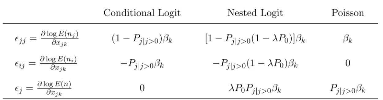
Table 1: Comparing implied elasticities (case A)
Conditional Logit Nested Logit Poisson jj = ∂log∂xE(nj)
jk (1−Pj|j>0)βk [1−Pj|j>0(1−λP0)]βk βk
ij = ∂log∂xEjk(ni) −Pj|j>0βk −Pj|j>0(1−λP0)βk 0
j = ∂log∂xEjk(n) 0 λP0Pj|j>0βk Pj|j>0βk
Notes: Pj|j>0 =E(nj)/E(n), P0 =E(n0)/E(n+n0)
taken by firms that would have chosen the outside option in the absence of a change in regional attractiveness.
2.1.4 A synthesis of the three models
We can now pull together the salient features of the three models. First, we consider the impact of a change in the attractiveness of an individual region on the number of firms in that region and across the J −1 remaining regions. Table 1 gathers the own-region, cross-region and aggregate elasticities implied by the three models.
In order to compare these elasticities, we define ρ = 1−λP0 which satisfies 0≥ ρ ≥ 1 under the standard nested logit assumption 0 < λ ≤1. We call ρ the rivalness parameter. It allows us to write the nested logit elasticities as a linear combination of their conditional logit and Poisson equivalents: nlogitjj =ρclogitjj + (1−ρ)jjPoisson, nlogitij =ρclogitij and nlogitj = (1−ρ)Poissonj . The rivalness parameter therefore acts as a summary measure of the position of the data generating process between the two polar cases, conditional logit (ρ= 1) and Poisson (ρ= 0). One may think ofρas capturing of the relative importance of the outside option: as ρ→ 0, competition among the J regions becomes unimportant relative to the weight of the outside option, while withρ→1, the outside option becomes negligible and any reallocations have to occur within the set of theJ regions.
We can also establish rankings of the elasticities implied by the three models. Provided thatβ 6= 0, the ranking of own-region elasticities is (c.f. Observations 2 and 6)
|Poissonjj |>|nlogitjj |>|clogitjj |>0,
while the ranking of cross-regions elasticities is just the reverse (c.f. Observations 3 and 6),
and the ranking of aggregate elasticities is again (c.f. Observations 4 and 7)
|Poissonj |>|nlogitj |>|clogitj |>0.
2.2 Case B: industry-specific locational determinants
Consider now that we observeK characteristicsxsj for every regionj and industrys. Hence,
we again do not observe firm-specific regional attributes, but we now allow for these attributes to differ acrossgroups of firms, best thought of as industries. We maintain the notation xj
for the subset of locational determinants that are constant across industries. Furthermore, njs is the number of firms in regionj and industrys,nsis the observed number of industry-s
firms across all regions, n is the total number of firms, and N stands for the corresponding observed firm count in the sample.
The grouped conditional logit model is given by the probability that a given firm f of industryschooses regionj rather than another region:
Pj|f =Pj|s = ex0sjβ PJ i=1ex 0 siβ , whereP
jPj|f = 1. Pj|s is the probability for a particular firm to choose region j given that
the firm belongs to industrys.
The grouped Poisson model is given by
E(nsj) =eαs+x
0 sjβ,
whereαs is an industry-specific constant.
Finally, the grouped nested logit model is given by the probability that a given firm f of industryschooses either the outside optionj= 0,
P0|s= eδs eδs + (PJ j=1e x0 sjγ/λ)λ = e δs eδs+ (PJ j=1e x0 sjβ)λ ,
or a particular domestic regionj >0,
Pj|s= ex0sjβ(PJ i=1ex 0 siβ)λ−1 eδs+ (PJ i=1ex 0 siβ)λ =Pj>0|s·Pj|j>0,s = (1−P0|s)Pj|j>0,s,
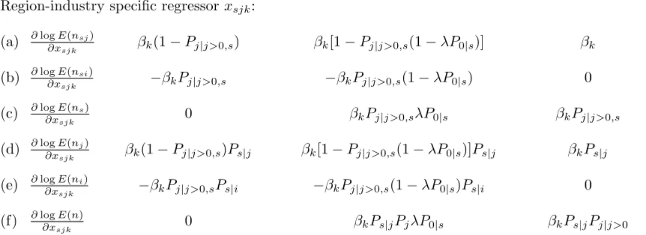
Table 2: Comparing implied elasticities (case B)
Conditional Logit Nested Logit Poisson
Region-industry specific regressorxsjk: (a) ∂logE(nsj) ∂xsjk βk(1−Pj|j>0,s) βk[1−Pj|j>0,s(1−λP0|s)] βk (b) ∂logE(nsi) ∂xsjk −βkPj|j>0,s −βkPj|j>0,s(1−λP0|s) 0 (c) ∂logE(ns) ∂xsjk 0 βkPj|j>0,sλP0|s βkPj|j>0,s (d) ∂logE(nj) ∂xsjk βk(1−Pj|j>0,s)Ps|j βk[1−Pj|j>0,s(1−λP0|s)]Ps|j βkPs|j (e) ∂logE(ni) ∂xsjk −βkPj|j>0,sPs|i −βkPj|j>0,s(1−λP0|s)Ps|i 0 (f) ∂log∂xE(n) sjk 0 βkPs|jPjλP0|s βkPs|jPj|j>0 Region specific regressorxjk:
(g) ∂logE(nj) ∂xjk βk PS s=1(1−Pj|j>0,s)Ps|j βkP S s=1[1−Pj|j>0,s(1−λP0|s)]Ps|j βk (h) ∂logE(ni) ∂xjk −βk PS s=1Pj|j>0,sPs|i −βkPSs=1Pj|j>0,s(1−λP0|s)Ps|i 0 (i) ∂log∂xE(n) jk 0 βkPj PS s=1(λP0|sPs|j) βkPj|j>0 Notes: Pj|j>0,s = E(nsj)/E(ns), P0|s = E(ns0)/E(ns+ns0), Ps|j = E(nsj)/E(nj). Ps|j is the fraction of firms in industrysin a given regionj.
that a given industry-sfirm chooses any domestic regionj >0,and
Pj|j>0,s = ex0sjβ PJ i=1ex 0 siβ (17)
is the probability that such a firm chooses a particular domestic region conditional on not choosing the outside option.
As in case A, the three models are observationally equivalent in a cross section of domestic firm choices and yield identical estimates for the parameter vector β. This has been shown by GFW for the grouped conditional logit and the grouped Poisson models, and we show it in the Appendix for the grouped nested logit model.
Table 2 summarizes the implied elasticities in the three grouped models (see the Ap-pendix for derivations). As in case A, the elasticities in the grouped nested logit model are (industry-specific) linear combinations of their conditional logit and Poisson equivalents: nlogit.. =ρsclogit.. + (1−ρs)Poisson.. whereρs= 1−λP0|s.
3
Estimation
3.1 Elasticity bounds
We have shown that estimation of any of the three models will yield identical parameter es-timatesβb. The additional parameters λ,δ and α in the nested logit model are not identified
but irrelevant for the estimation ofβ. Hence, it is impossible to discriminate formally between these three model based on cross-section data. And yet, the implied elasticities differ sub-stantially. In previous research, reported elasticities were based either on the conditional logit model or the Poisson model, without justification of the particular choice made or, mistakenly in this respect, by referring to the equivalence of the two models as established by GFW.
What can researchers do if they are not willing to make this choice by assumption but rely on cross-sectional data? We propose in this situation that one calculate the elasticities of both the conditional logit and the Poisson model and report these predictions as bounds for the true effects. As shown in Observation 6, intermediate values can be rationalized by a nested logit model.
The computation of both conditional logit and Poisson elasticities requires that one calcu-late predicted probabilities. In terms of case A (Table 1), the predicted probability is obtained as follows: ˆ Pj|j>0 = ex0jβˆ PJ i=1ex 0 iβˆ , (18)
while for case B (Table 2), there are three predicted probabilities to be computed:
ˆ Pj|j>0,s = ex0sjβˆ PJ i=1ex 0 siβˆ , (19) ˆ Ps|j = ex0sjβˆ PS r=1e x0rjβˆ , and (20) ˆ Pj|j>0 = PS r=1e x0 rjβˆ PS r=1 PJ i=1ex 0 riβˆ . (21) 3.2 An example
By way of an illustration, we take the data on location choices in Portugal by foreign-owned plants used in Guimaraes et al. (2000, 2003), and we report the elasticities implied by the coefficients of their regression model. The data cover a cross section of 758 location choices among 275 Portuguese regions by firms belonging to one of 151 industries.10 Their region-industry level regressor of main interest,xsjk, is “industry-specific agglomeration”, defined as 10We follow GFW by referring to industry-year pairs as “industries”. The 151 industries in their data set are combinations of 27 three-digit manufacturing sectors and seven sample years, ranging from 1985 to 1991.
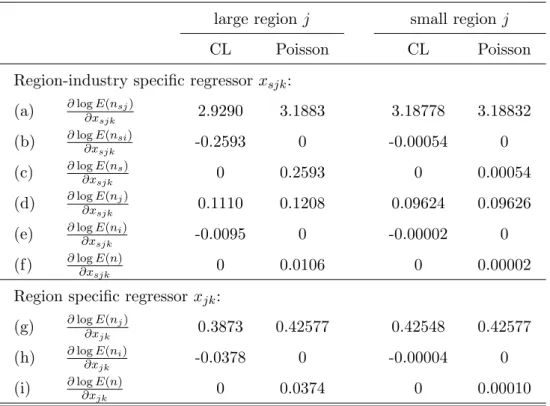
Table 3: Comparing implied elasticities in an example of case B
large regionj small region j
CL Poisson CL Poisson
Region-industry specific regressor xsjk:
(a) ∂logE(nsj) ∂xsjk 2.9290 3.1883 3.18778 3.18832 (b) ∂logE(nsi) ∂xsjk -0.2593 0 -0.00054 0 (c) ∂logE(ns) ∂xsjk 0 0.2593 0 0.00054 (d) ∂logE(nj) ∂xsjk 0.1110 0.1208 0.09624 0.09626 (e) ∂logE(ni) ∂xsjk -0.0095 0 -0.00002 0 (f) ∂log∂xE(n) sjk 0 0.0106 0 0.00002
Region specific regressor xjk:
(g) ∂logE(nj) ∂xjk 0.3873 0.42577 0.42548 0.42577 (h) ∂logE(ni) ∂xjk -0.0378 0 -0.00004 0 (i) ∂log∂xE(n) jk 0 0.0374 0 0.00010
Notes: large region: j= Lisbon; small region: j= Oleiros;i= Porto in rows (e) and (h); k = “industry-specific agglomeration” in rows (a) to (f), k= “total manufacturing agglomeration” in rows (g) to (i); sector: s= ISIC 351 (Industrial Chemicals) in 1989 in rows (a) to (f); any sector in rows (g) to (i).
the share of regional employment in the same industry as the relevant firm. Their region level regressor of main interest,xjk, is “total manufacturing agglomeration”, defined as the log of
aggregate manufacturing employment per square kilometer.
Taking their estimated parameters and computing the empirical probabilities (18)-(21), we can calculate all the implied elasticities of Table 2. Since the probabilities (18)-(21) vary by region and industry, we need to select specific cases for the computation of elasticities. We provide illustrations for two base regionsj: Lisbon, the largest region in terms of ˆPj|j>0, and Oleiros, the smallest region in terms of ˆPj|j>0 that still had non-zero firm counts in the larger industry considered.11
Table 3 shows the implied elasticities for changes in a region-industry specific regressor and in a region specific regressor. We can take these estimates to illustrate Observations 2 to 4.
• Observation 2: Own-region elasticities are larger in the Poisson model than in the
11
Where a comparison region ineeds to be specified for the computation of cross elasticities, we choose Porto, the second largest region in the data set. Where an industry s needs to be specified, we choose Industrial Chemicals (ISIC 351) in 1989, the largest sector-year pair in the dataset (31 observed choices, i.e. 4 percent of the total of 758 choices).
conditional logit (rows (a), (d) and (g)). We can see that the difference between implied own-region elasticities is non-trivial for the large region (some 10 percent) but very small for the small region (less than 0.1 percent). This illustrates that the difference between implied own-region elasticities of the two models vanishes as the number of regions grows large and individual regions therefore become small.
• Observation 3: All Poisson cross-region elasticities are zero (rows (b), (e) and (h)).
• Observation 4: In the conditional logit model, the total number of firms (across all of Portugal) is invariant to changes in the values of xsjk or xjk whereas in the Poisson
model the total changes with xsjk orxjk (rows (c), (f) and (i)). The effect on the total
number of firms of a given change in xsjk is stronger if the change occurs in a large
region.
These computations illustrate the qualitatively different predictions implied by the condi-tional logit and Poisson models. With J = 275 spatial alternatives and s = 151 industries, the underlying data set is highly disaggregated, implying relatively modest quantitative dif-ferences between implied elasticities. Nonetheless, even here some of the difdif-ferences are far from negligible. Perhaps the most striking difference appears in row (c) of Table 3. A one-unit change inxsjk of Lisbon leaves the number of Portuguese plants in industry s unchanged in
the conditional logit framework, while it increases by up to 29 percent in the Poisson model. Policy makers ought not to ignore a difference of such magnitude.
4
Conclusions
We show that the three standard location choice models - conditional logit, nested logit and Poisson - are observationally equivalent in terms of cross-section estimation yet imply starkly different predictions.
Take a corporate tax cut in a particular region. Provided that this is perceived by firms as making that region more attractive, all three models imply that the region itself will see an increase in its number of firms. We show that the magnitude of the implied increase differs: it is largest if the world is properly represented by the Poisson model, smallest if the world conforms with the conditional logit, and somewhere in-between if the world is nested logit. In a Poisson world, the tax cut will have no impact on firm counts in any other of regions within the data set. It will, however, pull firms away from other regions in the conditional logit and the nested logit cases. As the total number of firms is fixed in the conditional logit, the sum of the firms pulled away from the other regions is the same as the increase in the number
of firms in the tax-cutting region itself. The nested logit again represents an intermediate case, with some of the attracted firms relocating from elsewhere within the data set, implying that regional corporate tax bases are “rival”; and some firms appearing from outside that set, implying a “non-rival” tax base. The same logic can be applied to residential choices of private households with respect, for instance, to changes in local property tax rates.
Empirical researchers should be aware of the interpretational ambiguity affecting estimated parameters in standard location choice models, particularly if the number of locations and industries distinguished in the data is small. It can therefore be useful to report both condi-tional logit and Poisson elasticity estimates as bounds on the effects implied by the estimated parameters.
References
[1] Arzaghi, Mohammad and J. Vernon Henderson (2008) Networking off Madison Avenue. Review of Economic Studies, 75(4): 1011-1038.
[2] Bartik, Timothy J. (1985) Business Location Decisions in the United States: Estimates of the Effects of Unionization, Taxes and Other Characteristics of States. Journal of Business and Economic Statistics, 3(1): 14-22.
[3] Bayer, Patrick; Fernando Ferreira and Robert McMillan (2007) A Unified Framework for Measuring Preferences for Schools and Neighborhoods.Journal of Political Economy, 115(4): 588-638.
[4] Becker, Randy and Vernon Henderson (2000) Effects of Air Quality Regulations on Pol-luting Industries. Journal of Political Economy, 108(2): 379-421.
[5] B¨orsch-Supan, Axel (1990) Education and its Double-Edged Impact on Mobility. Eco-nomics of Education Review, 9(1): 39-53.
[6] Br¨ulhart, Marius; Mario Jametti and Kurt Schmidheiny (2007) Do Agglomeration Economies Reduce the Sensitivity of Firm Location to Tax Differentials? CEPR Dis-cussion Paper #6609.
[7] Carlton, Dennis W. (1983) The Location and Employment Choices of New Firms: An Econometric Model with Discrete and Continuous Endogenous Variables.Review of Eco-nomics and Statistics, 65: 440-449.
[8] Chirinko, Robert S. and Daniel J. Wilson (2008) State Investment Tax Incentives: A Zero-Sum Game? Journal of Public Economics, 92(12): 2362-2384.
[9] Coeurdacier, Nicolas; Roberto A. De Santis and Antonin Aviat (2009) Cross-Border Mergers and Acquisitions and European Integration. Economic Policy, 24(57): 55-106. [10] Crozet, Matthieu; Thierry Mayer and Jean-Louis Mucchielli (2004) How Do Firms
Ag-glomerate? A Study of FDI in France. Regional Science and Urban Economics, 34(1): 27-54.
[11] Davis, James C. and J. Vernon Henderson (2008) The Agglomeration of Headquarters. Regional Science and Urban Economics, 38(5): 445-460.
[12] Devereux, Michael P.; Rachel Griffith and Helen Simpson (2007) Firm Location Decisions, Regional Grants and Agglomeration Externalities.Journal of Public Economics, 91(3-4): 413-435.
[13] Duranton, Gilles; Laurent Gobillon and Henry G. Overman (2006) Assessing the Effects of Local Taxation Using Microgeographic Data. CEPR Discussion Paper #5856. [14] Ellickson, Bryan (1981) An Alternative Test of the Hedonic Theory of Housing Markets.
Journal of Urban Economics, 9(1): 56-79.
[15] Flowerdew, Robin and Murray Aitkin (1982) A Method of Fitting the Gravity Model Based on the Poisson Distribution.Journal of Regional Science, 22(2): 191-202.
[16] Greenstone, Michael and Enrico Moretti (2003) Bidding for Industrial Plants: Does Winning a ‘Million Dollar Plant’ Increase Welfare? NBER Working Paper #9844. [17] Guimaraes, Paulo; Oct´avio Figueiredo and Douglas Woodward (2000) Agglomeration
and the Location of Foreign Direct Investment in Portugal.Journal of Urban Economics, 47(1): 115-135.
[18] Guimaraes, Paulo; Oct´avio Figueiredo and Douglas Woodward (2003) A Tractable Ap-proach to the Firm Location Decision Problem. Review of Economics and Statistics, 85(1): 201-204.
[19] Guimaraes, Paulo; Oct´avio Figueiredo and Douglas Woodward (2004) Industrial Loca-tion Modelling: Extending the Random Utility Framework.Journal of Regional Science, 44(1): 1-20.
[20] Head, Keith and Thierry Mayer (2004) Market Potential and the Location of Japanese Investment in the European Union. Review of Economics and Statistics, 86(2): 959-972. [21] Head, Keith; John Ries and Deborah L. Swenson (1995) Agglomeration Benefits and Lo-cation Choice: Evidence from Japanese Manufacturing Investment in the United States. Journal of International Economics, 38(3-4): 223-247.
[22] Holl, Adelheid (2004) Manufacturing Location and Impacts of Road Transport Infras-tructure: Empirical Evidence from Spain.Regional Science and Urban Economics, 34(3): 341-363.
[23] List, John A. (2001) US County-Level Determinants of Inbound FDI: Evidence from a Two-Step Modified Count Data Model.International Journal of Industrial Organization, 19: 953-973.
[24] McFadden, Daniel (1974) Conditional Logit Analysis of Qualitative Choice Behavior. In P. Zarembka (ed.) Frontiers in Econometrics, New York: Academic Press, 105-142. [25] McFadden, Daniel (1978), Modelling the Choice of Residential Location. In A. Karlqvist
et al. (ed.)Spatial Interaction Theory and Planning Models, Amsterdam: North-Holland. [26] Nechyba, Thomas J. and Robert P. Strauss (1998) Community Choice and Local Public Services: A Discrete Choice Approach. Regional Science and Urban Economics, 28(1): 51-73.
[27] Papke, Leslie E. (1991) Interstate Business Tax Differentials and New Firm Location: Evidence from Panel Data. Journal of Public Economics, 45(1): 47-68.
[28] Quigley, John M. (1985) Consumer Choice of Dwelling, Neighborhood and Public Ser-vices.Regional Science and Urban Economics, 15(1): 41-63.
[29] Schmidheiny, Kurt (2006) Income Segregation and Local Progressive Taxation: Empirical Evidence from Switzerland.Journal of Public Economics, 90(3): 429-458.
[30] Wilson, Daniel J. (2009) beggar thy Neighbor? The In-State, Out-of-State, and Aggre-gate Effects of R&D Tax Credits.Review of Economics and Statistics, 91(2): 431-436.
Appendix: Derivations for case B Grouped conditional logit
The conditional logit model forgrouped data is given by the probability that a given firm f of industryschooses region j
Pj|f =Pj|s= ex0sjβ PJ i=1ex 0 siβ . The log likelihood function is
logL(β) = S X s=1 J X j=1 NsjPj|s = S X s=1 J X j=1 Nsjx0sjβ− J X j=1 [Nsjlog J X i=1 ex0siβ] .
The expected number of firms in regionj and industry sis E(nsj) =nsPj|s= nsex 0 sjβ PJ i=1ex 0 siβ .
and the corresponding own-region and cross-region elasticities within industrys are, respec-tively, ∂logE(nsj) ∂xsjk = (1−Pj|s)βk, ∂logE(nsi) ∂xsjk =−Pj|sβk.
The expected number of firms in industrysis
E(ns) = J
X
j=1
E(nsj) =ns=Ns,
and the corresponding elasticity within industrysis ∂logE(ns)
∂xsjk
= 0. The expected number of firms in regionj is
E(nj) = S X s=1 E(nsj) = S X s=1 nsPj|s= S X s=1 nsex 0 sjβ PJ i=1ex 0 siβ .
The corresponding own-region and cross-region elasticities are for a region-industry specific shockxsjk are ∂logE(nj) ∂xsjk = ∂logE(nsj) ∂xsjk ·E(nsj) E(nj) = (1−Pj|s)Ps|jβk, ∂logE(ni) ∂xsjk = ∂logE(nsi) ∂xsjk ·E(nsi) E(ni) =−Pj|sPs|iβk, wherePs|j =E(nsj)/E(nj).
The own-region and cross-region elasticities for a region-specific shockxjk are
∂logE(nj) ∂xjk = S X s=1 ∂logE(nsj) ∂xjk ·E(nsj) E(nj) =βk S X s=1 (1−Pj|s)Ps|j,
∂logE(ni) ∂xjk = S X s=1 ∂logE(nsi) ∂xjk ·E(nsi) E(ni) =−βk S X s=1 Pj|sPs|i.
The expected total number of firms in all regions and industries is
E(n) = S X s=1 J X j=1 E(njs) = S X s=1 E(ns) =n,
and the corresponding elasticities for a region-industry specific shockxsjk and a region-specific
shockxjk are, respectively,
∂logE(n) ∂xsjk = 0, ∂logE(n) ∂xjk = 0. Grouped Poisson
The Poisson model for grouped data is given as
E(nsj) =λsj =eαs+x
0 sjβ,
whereαs is an industry-specific constant. The concentrated log likelihood function is
logL(β) = S X s=1 J X j=1 Nsjx0iβ− J X j=1 [Nsjlog( J X i=1 ex0siβ)]− J X j=1 logNsj! +NslogNs −N.
The share of firms in regionj for any given industry sis given by Pj|s= E(nsj) PJ i=1E(nsj) = e αs+x0sjβ PJ i=1eαs+x 0 siβ = e x0 sjβ PJ i=1ex 0 siβ . The own-region and cross-region elasticities within industrysare, respectively,
∂logE(nsj) ∂xsjk =βk, ∂logE(nsi) ∂xsjk = 0. The expected number of firms in industrysis
E(ns) = J X i=1 E(nsi) = J X i=1 eαs+x0siβ = J X i=1 E(nsi) = J X i=1 eαs+x0siβ =eαs J X i=1 ex0siβ,
and the corresponding elasticity within industrysis ∂logE(ns) ∂xsjk = e x0sj PJ i=1ex 0 siβ βk=Pj|sβk.
The expected number of firms in regionj is
E(nj) = S X s=1 E(nsj) = S X s=1 eαs+x0siβ.
xsjk are ∂logE(nj) ∂xsjk = ∂logE(nsj) ∂xsjk ·E(nsj) E(nj) =Ps|jβk, ∂logE(ni) ∂xsjk = ∂logE(nsi) ∂xsjk ·E(nsi) E(ni) = 0, wherePs|j =E(nsj)/E(nj).
The own-region and cross-region elasticities for a region-specific shockxjk are
∂logE(nj) ∂xjk = S X s=1 ∂logE(nsj) ∂xjk ·E(nsj) E(nj) =βk, ∂logE(ni) ∂xjk = S X s=1 ∂logE(nsi) ∂xjk ·E(nsi) E(ni) = 0. The expected total number of firms in all regions and industries is
E(n) = S X s=1 J X j=1 E(njs) = S X s=1 E(ns) = S X s=1 " eαs J X i=1 ex0siβ # ,
and the corresponding elasticities for a region-industry specific shockxsjk and a region-specific
shockxjk are, respectively,
∂logE(n) ∂xsjk = ∂logE(nsj) ∂xsjk ·E(nsj) E(n) =Ps|jPjβk, ∂logE(n) ∂xjk = ∂logE(nj) ∂xjk ·E(nj) E(n) =Pjβk, wherePj =E(nj)/E(n).
Grouped nested logit
The nested logit model forgrouped data is given by the probability that firmf of industry s chooses the outside optionj = 0 or regionj >0 :
P0|s= eδs eδs + (PJ j=1e x0sjγ/λ)λ = eδs eδs+ (PJ j=1e x0sjβ)λ, Pj|s= ex0sjβ(PJ i=1ex 0 siβ)λ−1 eδs+ (PJ i=1ex 0 siβ)λ =Pj>0|s·Pj|j>0,s = (1−P0|s)Pj|j>0,s,
whereδs is an industry-specific constant, β =γ/λand
Pj|j>0,s = ex0sjβ PJ i=1ex 0 siβ . The concentrated log likelihood function is
logL(β) = S X s=1 J X j=1 Nsjx0sjβ− J X j=1 [Nsjlog J X i=1 ex0siβ]
+ Ns0log(Ns0) +Nslog(Ns)−(Ns+Ns0) log(Ns+Ns0)}. The expected number of firms in domestic regionj >0 and industrysis
and the corresponding own-region and cross-region elasticities within industrys are, respec-tively, ∂logE(nsj) ∂xsjk = [1−Pj|j>0,s(1−λP0|s)]βk, ∂logE(nsi) ∂xsjk =−Pj|j>0,s(1−λP0|s)βk.
The expected number of all domestic firms in industrysis
E(ns) = J
X
j=1
E(nsj) = (ns+ns0)(1−P0|s),
and the corresponding elasticity within industrysis ∂logE(ns)
∂xsjk
=λP0|sPj|j>0,sβk.
The expected number of firms in domestic regionj is
E(nj) = S X s=1 E(nsj) = S X s=1 (ns+ns0)Pj|s.
The corresponding own-region and cross-region elasticities for a region-industry specific shock xsjk are ∂logE(nj) ∂xsjk = ∂logE(nsj) ∂xsjk ·E(nsj) E(nj) = [1−Pj|j>0,s(1−λP0|s)]Ps|jβk, ∂logE(ni) ∂xsjk = ∂logE(nsi) ∂xsjk ·E(nsi) E(ni) =−Pj|j>0,s(1−λP0|s)Ps|iβk, wherePs|j =E(nsj)/E(nj).
The own-region and cross-region elasticities for a region-specific shockxjk are
∂logE(nj) ∂xjk = S X s=1 ∂logE(nsj) ∂xjk ·E(nsj) E(nj) =βk S X s=1 [1−Pj|j>0,s(1−λP0|s)]Ps|j, ∂logE(ni) ∂xjk = S X s=1 ∂logE(nsi) ∂xjk ·E(nsi) E(ni) =−βk S X s=1 Pj|j>0,s(1−λP0|s)Ps|i.
The expected total number of firms in all domestic regions and industries is
E(n) = S X s=1 J X j=1 E(njs) = J X j=1 E(nj),
and the corresponding elasticities for a region-industry specific shockxsjk and a region-specific
shockxjk are, respectively,
∂logE(n) ∂xsjk = ∂logE(nsj) ∂xsjk + X i6=j,i>0 ∂logE(nsi) ∂xsjk · E(nsj) E(n) =βkλP0|sPs|jPj, ∂logE(n) ∂xjk = ∂logE(nj) ∂xjk + X i6=j,i>0 ∂logE(ni) ∂xjk · E(nj) E(n) =βkPj S X s=1 (λP0|sPs|j), wherePj =E(nj)/E(n).