A Disciplined Option Writing Strategy Outperforms a Passive Dow 30 Total Return Index

(1)

A Disciplined Option Writing Strategy Outperforms a Passive Dow 30 Total Return Index

By Seth Allen and Henry Young

September 2011

Abstract

We have tested a simple option strategy of writing cash collaterized puts and covered calls based on data provided by the IVY Option Metrics Database. This database contains the actual put and call prices from December 31, 1995 to December 31 2010 used in this study. Our base case period for our option strategy (December 31, 1999 to December 31, 2010) has resulted in annualized returns ranging from 5.08% to 5.88% depending upon which P/E multiple cut off we used in our model. Comparatively, the DJIA delivered investors a total return of only 2.41%. Furthermore, our strategy, depending on the P/E cut-off, produced a standard deviation ranging from 4.06% to 5.99% versus the DJIA which had a considerably higher standard deviation of 15.77% for the same period measured. Our results beg the question: on a risk adjusted basis is writing of puts and calls a better strategy than simply investing in a passive index such as the Dow 30 index? The portfolio started with a notional $225,000 investment so as to compare it to a passive index investing strategy. The advantage of a simple, non-levered options writing strategy are significant as it handily outperforms a non-options passive index approach when measured on a risk adjusted basis.

(2)

Acknowledgements

We are appreciative and wish to thank Marko Ferenc, Gary Huebner, and Peter Klein for their helpful discussions and suggestions with regards to the design and accuracy of our model and approach.

(3)

Table of Contents:

Abstract………...1

Acknowledgements………...2

Section 1- Introduction………...………4

Section 2- Literature Review………...…………7

Section 3-Background on Put/ Covered Call Writing, and our Strategy…………...….13

Section 4- Methodology and Calculation of Returns………...……16

Section 5- Examination and Discussion of Empirical Results………...…………..25

Section 6- Conclusion………...…….59

Section 7.1- References………..………..61

(4)

Section 1-Introduction

It has been the desire of countless market practitioners to find ways to systematically “beat the market”. The question of whether a passive buy and hold strategy is better than an active strategy has been an ongoing debate for decades. Burton Malkiel, in writing the book “A Random Walk Down Wall Street”, concluded that outperforming the benchmark over the long run was unlikely. In our paper, we have put together a simple put/call option writing strategy that not only outperforms the underlying index in most cases, but does so with significantly less risk. Our base case time period (December 31, 1999 to December 31, 2010) handsomely outperforms the Dow 30 index with substantially less risk. The idea of more return with less risk is an utopian concept among market participants. Yet, we prove that a disciplined and patient rules-based option writing strategy achieves this advantage relative to a traditional buy and hold approach.

For the passive investor, the last decade has been less than stellar in terms risk and reward. The Dow Jones Industrial Average (DJIA) index started the year 2000 at 11,497.12 points and ended December 31, 2009 at 10,428.05, a drop of 9.30%. Even taking into account dividends (and not including annual management fees charged by ETF’s), the total return for the DJIA produced only a 1.31% nominal annualized return while having a standard deviation of 15.67% (source data: Bloomberg).

(5)

was to find a strategy that could cope with low market returns and high volatility while earning an individual investor a meaningful return on a risk adjusted basis.

For this project, we used the monthly data for the DJIA from December 31, 1995 to December 31, 2010. We examine several time periods over this fifteen year span to look at how the option strategy fared relative to the DJIA both in terms of return and volatility.

These Time periods include:

1. Our base case Dec 31, 1999 to December 31, 2010;

2. December 31, 1995 to December 31, 2010; 3. December 31, 1999 to December 31, 2008; 4. December 31,1999 to December 31, 2002; 5. December 31, 2002 to December 31, 2007; 6. December 31, 2007 to December 31 2010;

Between the time period December 31, 1995 to December 31, 2010, our option strategy encompassed some extreme macro events that ranged over bear, bull, and flat markets. These macro events include: the tech boom and bust, Asian currency crisis, Long Term Capital Management’s bankruptcy, Russian sovereign default, September 11th

, the housing bubble, wars in Iraq and Afghanistan, the Credit Crisis, and most recently the sovereign debt crisis (still ongoing) when this paper was written. What were some of the most turbulent times in the markets since the 1960’s and 70’s, our robust option strategy not only consistently holds up, but in most cases performed better when compared to the passive DJIA index investor both on an

(6)

absolute and risk adjusted basis. As illustrated below our base case time period using a 40x’s price to earnings (P/E) cut-off materially outperforms the Dow index.

Model Portfolio Growth vs. Dow 30 Index December 31, 1999 to December 31, 2010

Our strategy is rules based and we tested it over various scenarios. Specifically, we looked at various time periods but also with different P/E ratio cut-offs, dividend rates, interest rates, and minimum premiums required to see whether our thesis remains intact over these various scenarios.

Our strategy does not use any actual or implied leverage. The risk of bankruptcy is assumed to not exist. As well, so as to cash collateralize/cash secure our option writing strategy, the model carries a varying cash position that only earns the interest at the one year federal treasury rate

$0 $50,000 $100,000 $150,000 $200,000 $250,000 $300,000 $350,000 $400,000 $450,000 01 -Dec -99 01 -Dec -00 01 -Dec -01 01 -Dec -02 01 -Dec -03 01 -Dec -04 01 -Dec -05 01 -Dec -06 01 -Dec -07 01 -Dec -08 01 -Dec -09 01 -Dec -10 Portfolio DOW

(7)

The investment decision making process is rules based and so lacks the bias of subjective investor emotionalism when deciding to write an option and which options series to select. It is also important to note that our strategy/tool is not meant to forecast future markets but simply to react to them as our rules dictate.

The remainder of the paper is organized as follows. Section 2 is the literature review. Section 3 provides some background on put/call writing and our writing strategy. The methodology and calculation of returns is covered in Section 4. In Section 5, the empirical results are described for the base case scenario along with discussion of deviations from it. Section 6 provides conclusions of the paper and Section 7 contains the references and the appendix.

Section 2-Literature Review

The papers in our literature review were chosen to back up our position that options are more expensive than what their theoretical cost should be. Therefore, we believe an option writer can earn real income by collecting these overpriced premiums.

Bondarenko (2003) points to three reasons of why this is.

“E1: Risk premium. According to this explanation, high prices of puts are expected and reflect normal risk premiums under some equilibrium model. Even though the standard models cannot explain the data, maybe there is another model what can. In this “true” model, investors strongly dislike negative returns of the S&P Index and are willing to pay hefty premiums for portfolio insurance offered by puts.

(8)

E2: The Peso problem. According to this explanation, the sample under investigation is affected by the Peso problem. The Peso problem refers to a situation when a rare but influential event could have reasonably happened but did not happen in the sample. To illustrate this explanation, suppose that the market crashes (similar to that of October 1987) occur on average once in 5 years. Suppose also that investors correctly incorporate a probability of another crash in option prices. However, since only one market crash has actually happened over the studied 14-year period, the ex post realized returns of the Index are different from investors’ ex ante beliefs. In this case, puts only appear overpriced. The mispricing would have disappeared if data for a much longer period were available.

E3: Biased beliefs. According to this explanation, investors’ subjective beliefs are mistaken. Similar to E2, this explanation states that the Index realized returns have not been anticipated by investors. Consider an example. Suppose that the true probability of a crash in a given year is 20%, but investors incorrectly believe that this probability is 40%. Since investors overstate probabilities of negative returns, puts (especially OTM puts) are too expensive.” (Bondarenko, 2003, p. 1-2).

The point made in E1 is further strengthened by Garleanu, Pedersen, and Poteshman (2006). In their paper, they actually develop a model to test demand pressure on option prices. As noted in their paper, “intermediaries such as market-makers provide liquidity to end-users by taking the

(9)

Black-Scholes-Merton economy, then option prices are determined by no-arbitrage and demand pressure has no effect. In reality, however, even intermediaries cannot hedge options perfectly; that is, even they face incomplete markets because of the impossibility of trading continuously, stochastic volatility, jumps in the underlying, and transaction costs. In addition, intermediaries are sensitive to risk, e.g., because of capital constraints and agency.” (Garleanu et al, 2006, p.4260).

Garleanu, Pedersen, and Poteshman (2006) conclude that “we compute equilibrium prices as a function of net end-user demand and show that demand for an option increases its price by an amount proportional to the variance of the unhedgeable part of the option and that it changes the prices of other options on the same underlying asset by an amount proportional to the covariance of their unhedgeable parts.” (Garleanu et al, 2006, p.4293).

Ungar and Moran (2009), suggest that one can take advantage of overpriced put options and use it to gain excess returns. Their paper compares the performance and risk of a strategy that involves the cash-secured sales of at-the-money, S&P 500 Index put options, the CBOE S&P 500 PutWrite Index (ticker PUT). Unger and Moran (2009) state, “over a period of more than 22 years, the PUT Index has generated compound annual returns in excess of the S&P 500 Total Return Index, with 39% less volatility.”

(10)

Their paper also shows that the PUT Index outperforms the S&P 500 Total Return Index during bear and flat markets and underperforms during the bull markets as can be seen in Exhibit 1 (Bull Market Performance July 1994 – March 2000). This paper also goes into great detail to explain the practical reason why put premiums are so expensive. Mainly, it is cheaper for portfolio managers to buy put options than to sell off their whole portfolio when they are worried about the market entering a down turn. This is because it would entail huge transaction costs to exit out and re-enter the positions. There is also the risk that if they did not time the market correctly, they would be in double jeopardy as they would have liquidated their portfolio and would have to buy back all the positions at a much higher price. Their analogy is similar to “flood-insurance” policy holders, who are willing to renew policies ad infinitum without ever filing a claim.” (Ungar and Moran, 2009, p.53).

(11)

One of the most revealing points in the paper is Exhibit 2. The diagram shows that a “traditional allocation of 60% stocks and 40% bonds, which had a return of 8.8% and a standard deviation of 10.8%, when compared to a new option added allocation of 50% stocks, 30% bonds, and 20% PUT Index had a return of 9.5% and a standard deviation of 10.3%. The option-added allocation showed an improvement over the traditional allocation in that the option-added allocation had an annualized return that was 1.3% points higher and a standard deviation that was 0.5% points lower than the traditional allocation.” (Ungar and Moran, 2009, p. 51).

Exhibit 2

Exhibit 3 of Ungar and Moran (2009, page 54) show how the VIX, which measures the implied volatility of the S&P 500, is higher than the actual realized volatility of the S&P 500. This suggests that market participants are more fearful than they need to be. Therefore, option writers can demand a risk premium when they sell their options. In the next section of our paper we also

(12)

show this trend for the entire time series of our model and we also do this with the VXD, which is a measure of implied volatility of the Dow.

Exhibit 3

EnnisKnupp (2008) also examines the risk and returns of the CBOE S&P 500 PutWrite Index. A key point of why our model chooses to only write options with duration of six months or less can is explained on page 5. “The time decay of options accelerates as expiration approaches, with the time value of an option proportional to the square root of the portion of the year remaining until maturity. For example, a three-month option has half of the time premium of an option with four times the term, or one year, because the square root of one-quarter is one-half.” One criticism of this paper is that they are very light with their performance data. For example, nowhere in the paper do they address maximum drawdown and months to recover or the best or worst monthly returns. The paper also uses a poor representation of skewness and kurtosis in their results. They do not address the point that these statistical tests are not very relevant if you

(13)

do not have a normal distribution. Our paper will later discuss our own kurtosis and skewness results as we draw on the research of Brulhart and Klein’s (2005). Their paper sheds some evidence that although one can have high kurtosis and negative skewness, that this does not always equate to a situation where the fund is more risky than it is.

Section 3-Background on Put/Covered Call Writing, and our Strategy

The concept of options has existed since ancient times (Poitras, 2008). The buyer of an option contract receives the contractual right (but is not an obligation) to buy or sell an underlying asset at some future date. Conversely, the seller of the option contract may be obligated to deliver the underlying asset at some point in the future. The buyer of the option contract pays a premium to the seller to obtain this future right.

In 1973, Fischer Black and Myron Scholes developed the Black-Scholes (B/S) model for pricing of options, which for the first time allowed a market participant to quantify what an option should theoretically be worth. Since the 1970’s, options trading has expanded significantly and so have the multiple options trading strategies employed. Exotic names such as the Long Iron Butterfly or Iron Condor Spread are given to some of these more complex option combinations.

Many of these option strategies are sold to investors as conservative risk mitigating or hedged when in fact they are speculative. In some cases, when combined with other types of derivatives,

(14)

as described by Buffett, these are financial “weapons of mass destruction” as potential returns are much smaller than potential losses.

Conversely, our options strategy is based on some very simple value investment principles, which include the writing of put and call options on a cash collateralized basis. This strategy is the equivalent of bidding for a blue-chip stock materially below its current market price (put writing) or offering to sell a stock you own above its acquisition price (writing a covered call). Option writing, unlike straight equity purchases, has the added benefit of paying the investor non-refundable premiums for writing regardless of whether you buy/sell the actual underlying equity. Our strategy is to collect premiums from writing puts and, in the event of being put a position; we look to write a covered call on the stock we have acquired. All of these decisions are based on predetermined rules programmed into our algorithm. Once the rules are established for the algorithm, human emotion and subjective decision making is withdrawn from the investment process. Our strategy looks to write puts when stocks with a particular historic P/E ratio have sold off and to write covered calls when a stock (assuming we have been put the position) has recovered in price. In other words, we are using a value based contrarian approach famously described by Warren Buffett as “be greedy when others are fearful and be fearful when others are greedy”. Using options, we write puts when others are selling, and sell calls when investors are buying.

An obvious criticism regarding the effectiveness of our algorithm in identifying writing opportunities is that our model allows the user infinite variables in customizing an option writing

(15)

strategy. We have used historic data to back test how our option strategy would have performed over various time periods. We are acutely aware that the accusation of data snooping with our strategy is conceivable and therefore have kept the number of variables to only a few and our method for choosing them simple, intuitive, and realistic. This means we have used a combination of value investing principles along with actual observed practices by professional writers of options when choosing our variables. Thus we have been careful not to search endlessly for variables to fit our model, nor only look selectively at particular time periods that best suits our model.

Furthermore, we have run additional results on our model portfolio to deal with some of the more potentially contentious assumptions such as the assumed dividend rate, interest rate, minimum premium required, or time period chosen

Another obvious question to ask of our model is whether implied leverage is being used. In other words, are the positions that we are writing puts on truly cash secured? In all scenarios where the model used a maximum P/E ratio to write a put on an underlying equity there was always cash balances available to pay for the stock if it were assigned. When no P/E rule was applied some leverage (17% for time period December 31, 1995 to December 31, 2010) was employed but no bankruptcy occurred. We also have the ability to write a rule into the algorithm that regardless of whether our model indicates an option writing opportunity we have a “fail safe” in place that stops the model in those cases where cash collaterization of the portfolio falls below 100%.

(16)

Section 4.1-Methodology and Calculation of Returns

Our model is a rules based algorithm that identifies option writing opportunities. The data source for option pricing of puts/calls comes from the IVY Option Metrics Database. This database contains all put and call option prices going back to December 1995 for US traded options (this is as far back as the data goes). As the data is non-split adjusted, we accounted any splits that occurred during the period measured.

We used Bloomberg, Yahoo Finance, the Federal Reserve, and Thomson Reuters to source other return data such as the benchmark total return, historical dividend yields, historic P/E multiples, and interest rates.

The data once gathered was run through an off the shelf data processing program called SQL Server 2008. Microsoft Excel was then used to calculate our statistical results.

The following are the rules used by our model to generate our option writing opportunities:

A. Price to Earnings Multiple:

In our base case scenario we use a price to earnings multiple (P/E) of less than 40 P/E as the maximum multiple that we would write a put option on an underlying equity. For comparison purposes we have also looked at P/E multiples of less than 15, 20 and 30 times along with a no P/E cut-off scenario. We use trailing P/E multiples at the time observed which were provided by

(17)

Bloomberg. The reason for using P/E ratios to influence our put write decisions is to avoid writing on equities that are clearly over priced from a fundamental perspective the way, say, Cisco Systems was in October 2000 with a then current trailing P/E of 112. However, regardless of whether a no P/E rule is applied our model still outperformed the Dow with respect to risk and return in our base case scenario but lagged the returns of most of the other P/E cut-offs. The no P/E cut-off scenario also had the highest standard deviation when compared to implementing other earnings multiple thresholds. While a 30-40x’s P/E equity is hardly a “value” stock, the idea was to eliminate stocks that exhibit bubble-like, silly valuations that inevitably correct harshly. As well, this belief in avoiding over valued stocks is supported by Campbell and Shiller who concluded that overly high P/E multiples and low dividend yields lead to substantial equity losses in the years to follow (Campbell and Shiller, 1999).

B. Minimum Premium Required:

For writing a put/covered call, the minimum premium collected has to be greater than 3.9% in our base case. Although somewhat arbitrary, the reason for requiring a minimum premium of more than 3.9% is that on an annualized basis we are looking to receive a nominal return of approximately 8%. Given that we are looking to compare our model to a passive investor we believe that we need to get a minimum annual return that is comparable to what a long only equity investor should expect if we are to write a put and potentially own the underlying equity. As well, observations made of some professional market practitioners’ option writing generally reveal that in many cases the premiums required are indeed greater than 3.9% or they may feel that the return is not sufficient to justify the risk (Ferenc, 2010). Although we are comfortable with the minimum premium requirement of greater than 3.9%, we also ran our base case time

(18)

period (December 31, 1999 to December 31, 2010) with greater than 1.5%, 2.5% and 5% premium thresholds.

C. Maximum Duration of Option Contract:

The maximum term-to-expiry selectable by the model was capped at six months. The model selected the nearest month to achieve the stated premium threshold (e.g. 3.9%) at the lowest given strike price and not longer. As writers of options we want to maximize the value or time decay of Theta.

D. Stock Price:

Shares must be trading less than 85% of its 52 week rolling high. As our model has been constructed based on value investing, we believe that there should only be writing opportunities presented when an equity has “sold off”. A drop in a stock of 15% or more would be regarded as a correction and potential buying opportunity by market practitioners.

Only write a call if assigned/ put the stock; then write a covered call if:

1. A minimum premium greater than 3.9% can be collected. 2. The option contract is six months or less in duration.

3. The strike price of the covered call is at or above the price you were put the stock at.

Based on the above rules the algorithm generates a list of eligible equities and the model will pick the option with the lowest strike price.

(19)

The following assumptions are made:

A1. Interest Rate:

The interest rate earned from unused cash is based on the monthly yield of the one year treasury rate (see Table C in appendix) at the time. For comparison purposes, we also ran the model using a flat 1% rate for all periods.

B1. Dividend Rate:

For equities that get “put” we have assumed an average dividend rate received for the period held. The assumed dividend rate used in our base case is 2.9% annualized. Historically dividend yields have been 3% to 7% (Campbell and Shiller, 1999). For comparison purposes we ran our model using an assumed dividend rate of 1% and 0%.

C1.Equities Universe for Option Writing:

We have used the stocks that existed in the DJIA as of December 31, 2010.

D1. Portfolio Universe of Companies:

AA- Alcoa Inc.

AXP- American Express Company

BA- The Boeing Company

BAC- Bank of America Corp.

CAT- Caterpillar Inc.

(20)

CVX- Chevron Corp

DD- Dupont

DIS- The Walt Disney Company

GE- General Electric Company

HD- Home Depot Inc.

HPQ- Hewlett-Packard Company

IBM- International Business Machines

INTC- Intel Corp

JNJ- Johnson & Johnson

JPM- JP Morgan Chase & Company

KFT- Kraft Foods Inc.

KO- The Coca Cola Company

MCD- McDonalds Corp

MMM- 3m Company

MRK- Merck & Company Inc.

MSFT- Microsoft Corp

(21)

PG- The Procter & Gamble Company

T- AT&T Inc.

TRV- The Travelers Companies Inc.

UTX- United Technologies Corp

VZ- Verizon Communications

WMT- Wal Mart Stores Inc.

XOM- Exxon Mobil Corp

E1. Risk Free Rate:

The assumed risk free rate is 1%.

F1. Early exercise:

The options that we are writing are American style and could be exercised early. However, for purposes of this paper we have assumed that they are not exercised until maturity.

G1. Transaction Costs:

For the purpose of this paper we have left out transaction costs as they would not materially impact our results. Institutions typically pay $1.00 per board lot and trading commissions would be $10 or less per board lot traded. Our base case model would have incurred transactions costs of roughly $1400.00, which is not material to our overall returns.

(22)

H. Liquidity and Execution:

For the purposes of this paper we have assumed that when an option writing event is identified, we can execute at the quoted price at the time. We are only buying one board lot if put a position. Our data source only gives us bid/ask prices and we assume that we execute in the middle of the spread between the bid and ask price. Ideally we would want to use the volume weighted average price (VWAP), but this data was not available to us.

I1. Portfolio Size:

The starting portfolio value is $225,400 for our base case time period. The portfolio starting value is based on buying one board lot of each Dow stock at the closing prices as of December 31, 1999. The portfolio size changes depending on the starting time period so as to reflect the changing values of the Dow 30 stocks.

J. Number of Shares:

Our model will write one contract (equivalent to one board lot, or 100 shares) unless there are stock splits. For example, after a two-for-one stock split any subsequent trading events for that stock would then mean the model writes two contracts (or 200 shares).

K. Time Period Examined:

We examine six different time periods that reflect different market conditions encompassing bull and bear markets as temporary market corrections.

These periods include:

(23)

2. December 31, 1995 to December 31, 2010. Total period covered by the data. 3. December 31, 1999 to December 31, 2008. Bear Market.

4. December 31, 1999 to December 31, 2002. Bear Market 5. December 31, 2002 to December 31, 2007. Bull Market 6. December 31, 2007 to December 31 2010. Bear Market.

Section 4.2-Excess Return Computation

Our option writing strategy is structured so that cash is available at all times to pay for an equity if put the position. In our base case model that uses a P/E of 40 cut-off and time period December 31, 1999 to December 31, 2010, the maximum cash position used to purchase put equity positions was 36.07% of the portfolio. In other words, in August, 2009 the portfolio was 63.93% invested in one year federal treasuries and 36.07% invested in equities.

Measuring the excess return on our model can be based on a cash collaterized/committed basis or only when actual capital is invested in the model when put a position. When looking at measuring the excess return of the model portfolio we have opted to base it on cash collaterized/committed capital. We have also done this because it avoids using implied leverage. This means that our model is at all times able to pay in cash for every put equity position without needing to use margin borrowing to do so.

(24)

We also acknowledge that hedge funds and large institutions could implement our option writing strategy using capital only when the portfolio is put an equity position. The ability to source capital when needed is not necessarily easy for the retail investor nor would the implied leverage be necessarily manageable if all put positions were to be assigned simultaneously. Our base case has a large percentage of the portfolio in cash at all times during the measured time period and could lull the investor into believing that our strategy can handle leverage. As the past may not predict the future it would be dangerous to assume there could never be a market bearish enough to trigger assignments on all puts written. This possibility must always be respected. To reiterate, our model is a disciplined value based option writing strategy which is designed to outperform a passive buy/hold Dow 30 index investment with less risk and without leverage.

The total portfolio balance for the month consists of three separate components. The first component is the cash balance, which grows each month by the assumed cash interest rate. This cash component grows by the addition of any premiums that are collected for that month and by any securities that are sold. As well, the cash balance will decrease if the model is signalled to undergo a buy transaction due to a put option being exercised. The second component is the amount of option premiums that are collected from the writing of puts and calls. The third component is the value of the equity holdings, which will fluctuate depending on the market price of the securities. All three components are summarized in the below formula. We have calculated the returns for the model portfolio based on monthly data.

(25)

1. Monthly Portfolio Balance = Cash Balance*(Cash Interest Rate) + Option Premiums + Equity Balance

2. The monthly return is = (Monthly Balance – Previous Monthly Balance) / Previous Monthly Balance.

3. The portfolio’s cumulative returns is calculated by the formula = (1+Monthly Return) * Previous Month’s cumulative return.

4. Once we have the portfolio’s cumulative return, we can than find the annualized return with the following formula. Annualized return = (Portfolio’s Cumulative Return) ^ (12/number of months) -1.

5. Finally, the excess return is the portfolio’s annualized return less the risk free rate. The same process is also used to calculate the excess return of either the Dow or S&P.

Section 5-Examination and Discussion of Empirical Results

We ran our model starting with our base case time period of December 31, 1999 to December 31, 2010, P/E cut-off of less than 40, assumed dividend rate of 2.9%, minimum option premium required greater than 3.9%, historical interest rates and a portfolio size of $225,400 (Figures 1a and 1b).

We have also run our model with changes to assumed dividend rate, interest rate, minimum premiums required to write an option, and various time periods.

(26)

The below Figure 1a shows the detailed returns of what the model generates depending on what valuation (P/E) cut-off is used.

Figures 1a and 1b compares the results to the two benchmarks, which are the total return for the Dow 30 and the total return for the S&P 500 for the time period from December 31, 1999 to December 31, 2010. The S&P has been included for reference purposes only as the Dow 30 is the index that our model is being compared to.

Figure (1a) shows the performance of the base case time period.

Model NO PE 15 PE 20 PE 30 PE 40 PE DOW Total Return S&P 500 Total Return Starting Balance $225,402.00 $225,402.00 $225,402.00 $225,402.00 $225,402.00 $225,402.00 $225,402.00 Ending Balance $390,646.85 $371,709.77 $404,472.54 $415,547.01 $424,506.42 $292,843.61 $235,759.74 Since Inception 72.472% 64.111% 78.580% 83.465% 87.421% 29.921% 4.595% Annualized Return 5.080% 4.606% 5.413% 5.672% 5.877% 2.408% 0.409%

Best Month ROR 4.682% 4.758% 4.425% 4.576% 4.225% 10.844% 9.783%

Worst Month ROR -5.265% -5.036% -4.977% -4.946% -5.010% -13.884% -16.795%

Max Drawdown -17.379% -16.947% -16.816% -16.464% -16.089% -47.120% -50.920% Length of Drawdown May 2008 - Feb 2009 Aug 2008 - Feb 2009 Aug 2008 - Feb 2009 Aug 2008 - Feb 2009 Aug 2008 - Feb 2009 Oct 2007 - Feb 2009 Oct 2007 - Feb 2009 Months to Recover 9 9 9 9 9 Has not recovered Has not recovered

Figure (1b) shows the statistical results of the base case.

Model NO PE 15 PE 20 PE 30 PE 40 PE DOW Total Return S&P 500 Total Return Standard Deviation 5.993% 4.060% 4.162% 5.282% 5.236% 15.770% 16.409% Sharpe Ratio 0.681 0.888 1.060 0.873 0.931 0.089 -0.036

Jensen's AlphaDOW 3.643% 3.383% 4.160% 4.287% 4.508% na na

Jensen's AlphaS&P 4.253% 3.967% 4.513% 4.823% 5.022% na na

CorrelationDOW 0.816 0.616 0.680 0.805 0.789 na na

CorrelationS&P 0.800 0.618 0.671 0.783 0.769 na na

Kurtosis 1.719 9.035 6.999 2.388 2.616 0.597 0.628

(27)

When comparing the results from our model to the Dow and S&P indices our base case handily outperforms from a return and risk stand point. The P/E 40 cut-off delivers an annualized return of 5.88% with a standard deviation of 5.24% versus the Dow, which returns 2.41% annualized with a standard deviation of 15.77%. The S&P 500 has even worse performance when compared to the base case model with an annualized return of 0.41% and a standard deviation of 16.41%. As one can see, the model’s performance numbers are better than both benchmarks and these results were accomplished with a lower level of risk. The other P/E cut-offs also exhibited better returns (annualized returns of 4.61% to 5.67%) than the Dow and S&P along with less risk (standard deviations of 4.06% to 5.99%).

The base case model with a P/E 40 threshold had a correlation 0.79 to the Dow. The other P/E cut-offs for our base case have a correlation to the Dow ranging from 0.62 to 0.82.

Figure 1b also shows our model generating higher kurtosis and negative skewness along with a high Sharpe ratio, and positive Jensen’s Alpha. However, as the returns for our model are not normally distributed (see Figure 2a on page 30) some of our statistics including kurtosis, negative skewness, the Sharpe ratio, and Jensen’s Alpha, could lead to spurious conclusions about the true riskiness of the model.

With a normal distribution of returns, higher kurtosis denotes the possibility of extreme outlier returns and negative skewness indicates these extreme outlier returns to be negative. However,

(28)

Todd Bulhart and Peter Klein (2005) point out that when you have returns that are not normally distributed it would be misleading to believe that higher kurtosis and negative skewness implies greater risk. Bulhart and Klein point out that one method for observing the risk of an investment strategy that lacks a normal distribution of returns is to look at the magnitude of maximum drawdown and the number of months to recover.

The base case model (Figure 1a) peak-to-trough (August 2008 to February 2009) to recovery was -16.09% and nine months, respectively. The Dow peaked in October of 2007 with a maximum drawdown of -47.12% and still had neither recovered as of December 31, 2010 nor at the time of writing this paper in the fall of 2011. As well, the base case model experiences less volatility monthly with the worst month being 5.01% compared to the Dow’s worst month being down -13.88%. In the base case model the other P/E cut-offs had the same months to recover and similar worst/best month and maximum drawdown as the P/E 40 cut-off.

With respect to the Sharpe ratio and Jensen’s Alpha, indicated results in our base case model are good from a risk/reward standpoint and the appearance of beating the Dow 30 index. The Sharpe ratio in Figure 1b ranges from 0.68 to 1.06 depending on the P/E cut-off. The higher the Sharpe ratio number the better the investor is being compensated for the risk taken.

The Jensen’s Alpha in Figure 1b ranges from 3.64% to 4.51% depending on the P/E cut-off. Jensen’s Alpha looks at the extra return being generated on the model portfolio above what the

(29)

Capital Asset Pricing Model (CAPM) expected return should be for the model portfolio given the base case model portfolio beta.

For our Jensen’s Alpha, we ran a robustness check using the Fama and French three factors plus an additional momentum factor (MOM). This four factor model is known as the Carhart Four Factor model, which accounts for momentum in explaining stock market returns. In our base case, with a P/E 40 cut-off, our Jensen’s Alpha modestly drops (16% or 74 basis points) from 4.51% to 3.77%. The HML (high book-to-market minus low) factor contributed the most (.40%) to the drop in our Jensen’s Alpha. The other factors MOM and SMB (small market capitalization minus) contributed .13% and .21%, respectively. As our model is based on value investing, it would make sense that the HML factor would have some impact on our Jensen’s Alpha.

However, as our returns are not normally distributed, the Sharpe ratio and Jensen’s Alpha should not be considered exclusive of other meaningful statistics such as worst month, best month, maximum drawdown, and duration of drawdown.

Overall, the base case model for all P/E cut-offs generates returns that not only outperform the Dow in terms of total annualized returns, but does so with less risk.

(30)

Figure 2a shows the distribution of returns for our model. The best monthly return was 4.23% while worst monthly return was -5.01% versus the Dow with 10.84% and -13.88%, respectively.

(31)

Figure2(a) 0 5 10 15 20 25 30

Frequen

cy

Monthly Returns %

Portfolio Vs Dow

Portfolio

Dow

(32)

For our base case time period (December 31, 1999 to December 31, 2010) we have produced two charts from Bloomberg that show the implied volatility (VXD and VIX) versus the actual volatility experienced by the Dow and S&P indices. With model returns not normal (as shown in Figure 2a) and with the persistent spread between the actual versus implied volatility (as show in Figure 2b and Figure 2c) our results seem to coincide with the findings of other studies such as Ungar & Moran, (2009) and EnnisKnupp, (2008).

Although the purpose of this paper is to identify an options writing model that outperforms the Dow index on a risk adjusted basis, the implications of why this has occurred is important to a market participant going forward. The idea that this spread between implied versus actual volatility could continue to exist going forward suggests that option writing should remain profitable in practice. The chart below shows the VXD, which is the implied volatility of the Dow (orange line) versus the actual volatility of the Dow.

(33)

Figure 2(b)

(34)

The same trend is also observed when one overlays the VIX (orange line) with the actual volatility of the S&P Index (white line).

Figure 2(c)

Source: Bloomberg

The following is a summary of the actual transactions that the model executed over the base case time period (December 31, 1999 to December 31, 2010) with the P/E 40 cut-off. The model was the most active with the writing of options during years 2000, 2001, and 2008. This would make

(35)

sense as those years represent significant market volatility including the tech bubble, September 11th, and the Credit Crisis.

Total puts written: 217.

Total calls written: 100.

Total equity buys: 62.

Total equity sells: 48.

For a complete breakdown of every position that is either written/bought/sold please refer to Table A in the appendix.

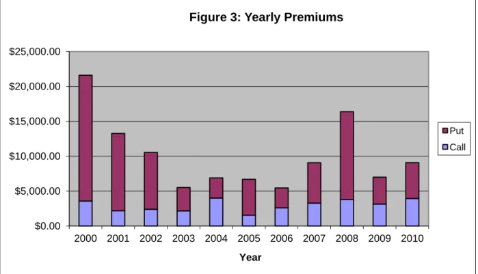
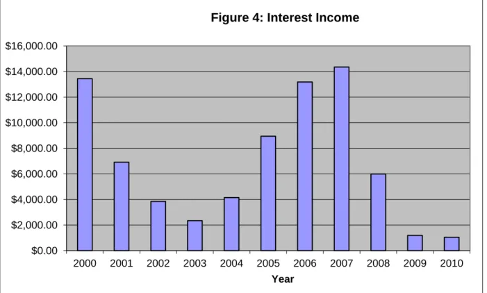
Figures 3, 4, 5, and 6 show the premiums, interest income, portfolio growth, and asset allocation over the base case time period.

(36)

Figure 4 shows the amount of interest income generated over the base case time period. When interest rates have declined significantly during the observed period, interest income will contribute less to the portfolio’s return as seen in years 2003, 2009, and 2010.

$0.00 $5,000.00 $10,000.00 $15,000.00 $20,000.00 $25,000.00 2000 2001 2002 2003 2004 2005 2006 2007 2008 2009 2010 Year

Figure 3: Yearly Premiums

Put Call

(37)

Figure 5 gives a graphical representation of the growth of the model portfolio versus the total return of the Dow index over the observed base case period.

$0.00 $2,000.00 $4,000.00 $6,000.00 $8,000.00 $10,000.00 $12,000.00 $14,000.00 $16,000.00 2000 2001 2002 2003 2004 2005 2006 2007 2008 2009 2010 Year

Figure 4: Interest Income

$0 $50,000 $100,000 $150,000 $200,000 $250,000 $300,000 $350,000 $400,000 $450,000 Dec -99 Dec -00 Dec -01 Dec -02 Dec -03 Dec -04 Dec -05 Dec -06 Dec -07 Dec -08 Dec -09 Dec -10 Portfolio DOW

(38)

Figure 6 shows the yearly cash and equity balances. After a major market downturn, such as in 2001-2003 and 2008-2009, there is an increase in equity holdings since the model is forced to pay for put assignments. During stable or bull markets the portfolio holds relatively high amounts of cash as the model sells off its equity positions when its covered calls are called away and is assigned less on the put side. Refer to Table B in the appendix to see the monthly portfolio holdings broken down into cash, interest, premiums collected, and equity balance. As well, the last column in Table B shows what percentage of the portfolio is cash.

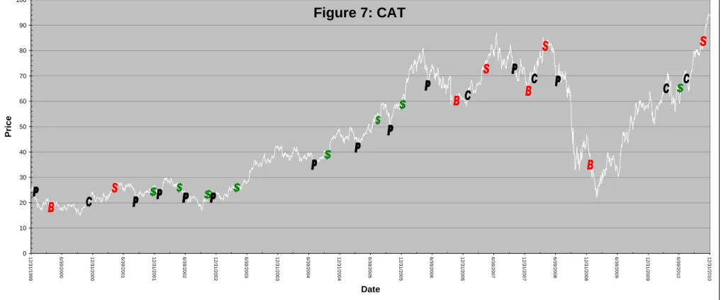
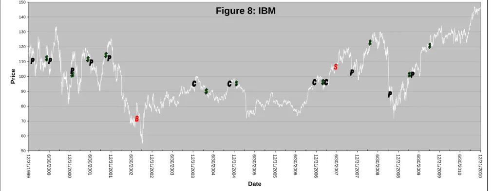
Figures 7 and 8 shows the specific transaction activity for two of the more active stocks for writing in our base case model portfolio: IBM and Caterpillar. The graphs show the equity price movements along with our model portfolio actions starting with when a put has been written.

$0.00 $50,000.00 $100,000.00 $150,000.00 $200,000.00 $250,000.00 $300,000.00 $350,000.00 $400,000.00 $450,000.00 2000 2001 2002 2003 2004 2005 2006 2007 2008 2009 2010

Figure 6: Portfolio Composition

EquityBalance CashBalance

(39)

Legend

B = Stock purchased as put option was assigned

P = Put was written

$ = Put or Call expired worthless, therefore, premium was kept

C = Call was written

S = Stock sold as call was assigned

Figure 7: CAT 0 10 20 30 40 50 60 70 80 90 100 12/ 31/ 1999 6/ 30/ 2000 12/ 31/ 2000 6/ 30/ 2001 12/ 31/ 2001 6/ 30/ 2002 12/ 31/ 2002 6/ 30/ 2003 12/ 31/ 2003 6/ 30/ 2004 12/ 31/ 2004 6/ 30/ 2005 12/ 31/ 2005 6/ 30/ 2006 12/ 31/ 2006 6/ 30/ 2007 12/ 31/ 2007 6/ 30/ 2008 12/ 31/ 2008 6/ 30/ 2009 12/ 31/ 2009 6/ 30/ 2010 12/ 31/ 2010 Date Pric e

(40)

Legend

B = stock purchased as put option was assigned

P = Put was written

$ = Put or Call expired worthless, therefore, premium was kept

C = Call was written

S = Stock sold as call was assigned

Figure 8: IBM 50 60 70 80 90 100 110 120 130 140 150 12/31/1999 6/30/2000 12/31/2000 6/30/2001 12/31/2001 6/30/2002 12/31/2002 6/30/2003 12/31/2003 6/30/2004 12/31/2004 6/30/2005 12/31/2005 6/30/2006 12/31/2006 6/30/2007 12/31/2007 6/30/2008 12/31/2008 6/30/2009 12/31/2009 6/30/2010 12/31/2010 Date Price

(41)

Figures 9, 10, 11, 12, 13, and 14 look at the base case time period of December 31, 1999 to December 31, 2010. Each scenario will have all variables kept the same with only one variable changed. Figure 9 deals with the scenario of how the model holds up if interest rates are kept at a static value of 1% for the observed time period. Figures 10 and 11 show the output from the model when only the dividend rate is modified (0% and 1%). Figures 12, 13, and 14 show the results from the model when only the minimum option premium rate is modified.

One can observe by comparing the results from Figures 9 to 11 that the model is more sensitive to cash interest rates than dividend rates. This can been seen in the reduction in the annualized returns and the increase in the standard deviation for all P/E cases when the interest rate has been dropped to 1%. In other words, with materially lower interest rates than the base case there has been less portfolio growth. When faced with maximum drawdown, the low interest scenario had less cash to cushion the decline in the equity portion of the asset composition. Interestingly the portfolio recovers in the same amount of time as the base case (nine months) regardless of interest rates or dividend yield applied as shown in Figures 9, 10, and 11.

Our base case P/E 40 cut-off annualized return goes from 5.88% to 4.66% (Figure 9a) when the interest rate is changed to 1%. There is less effect on the annualized returns when the assumed dividend rate of 1% and 0% is used. Figures 10a and 11a show the P/E 40 cut-off return being 5.47 and 5.25%, respectively.

(42)

The standard deviation increases in Figure 9b P/E 40 cut-off to 5.82% from the base case of 5.24%. For the dividend scenario in Figures 10a and 10b, the standard deviation barely changes. Coinciding with the higher standard deviation observed in Figure 9b is materially higher maximum drawdown of 18.71% with the 1% static interest rate scenario.

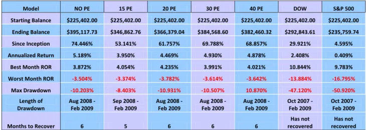
With the option premium thresholds for writing changed as seen in figures 12, 13, and 14, the total returns vary along with the riskiness of the model. When a P/E cut-off 40 is used the returns for 1.5% premium (Figure12a and 12b) are less. However, so is the standard deviation, while the maximum drawdown is 10.87% versus the base case of 16.09%. As well, it takes only six months to recover (as seen in Figure 12a) compared to the base case where it takes nine months to recover.

When looking at the 2.5% premium (Figure13a and Figures 13b) the returns are very close or the same as the base case along with the maximum drawdown, months to recover, and standard deviation.

With the 5.0% premium (Figure 15a and 15b) the returns and months to recover are nearly identical to the base case but other measures such as the maximum drawdown and standard deviation are materially higher.

(43)

It would seem that decreasing the interest rates (flat 1%) assumed and demanding a high premium (5%) does not increase the return but only the risk as shown by greater drawdowns and higher standard deviation. With dividends it does not seem to matter what rate is assumed as seen in Figures 10 and 11.

The Sharpe ratio and Jensen’s Alpha for the various P/E cut-offs in Figure 9b are lower than the base model but still show the model with static interest rates outperforming the Dow on a risk adjusted basis. As Figures 10b and 11b show, the Sharpe ratio and Jensen’s Alpha are less changed for the various P/E cut-offs but still outperforms the Dow on a risk adjusted basis.

Interestingly in Figure 12b, when the option premium required is changed to 1.5%, the Sharpe ratio rises significantly, ranging from 1.245 to 1.376 depending on which P/E cut-off is used. In fact when no P/E cut-off is used, it delivers the highest Sharpe ratio of 1.376.

The Jensen’s Alpha in Figure 12b also rises materially (4.013%) for the no P/E cut-off when compared to the no P/E off base case model in Figure 1b but does not exceed the P/E 40 cut-off in Figure 1b. Only when a P/E cut-cut-off (15, 20, 30, 40x’s) is applied in Figure 12b does the Jensen’s Alpha materially decrease as compared to the base case model.

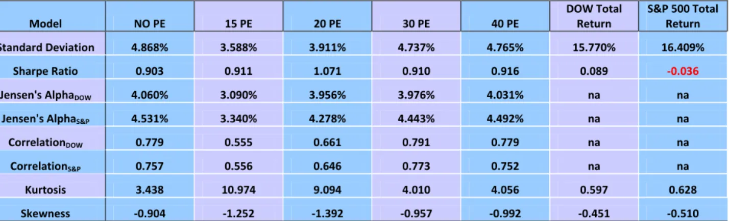
When the option premium is set at 2.5% as show in Figure 13b there is very little change compared to the base case for the Sharpe ratio when a P/E cut-off is applied. The Jensen’s

(44)

Alpha decreases with P/E cut-offs applied ranging from 3.09% to 4.03% versus the base case that ranges from 3.38% to 4.508% for the 15, 20, 30, and 40x’s P/E cut-offs, respectively.

When no P/E cut-off is used the Sharpe ratio rises to 0.903 versus 0.681 for the base case no P/E cut-off and Jensen’s Alpha increases to 4.06% versus the base case of 3.643%.

In Figure 14b, when the option premium is set at 5%, the Sharpe ratio and Jensen’s Alpha are relatively unchanged from the base case for various P/E cut-off scenarios.

Overall, the various scenarios in Figures 9, 10, 11, 12, 13, and 14 exhibit similar characteristics of outperforming the Dow 30 index in terms of total return on a risk adjusted basis. Interest rates on cash balances and option premiums required to write seem to have some effect on the risk adjusted returns when to compared to the base case model. However, dividend rates have a marginal impact on the risk adjusted returns.

(45)

Figure (9a) shows the performance of the base period December 31, 1999 to December 31, 2010 with the cash interest rate set to a static value of 1% for the observed period.

Model NO PE 15 PE 20 PE 30 PE 40 PE DOW Total Return S&P 500 Total Return Starting Balance $225,402.00 $225,402.00 $225,402.00 $225,402.00 $225,402.00 $225,402.00 $225,402.00 Ending Balance $343,942.07 $315,026.12 $347,496.61 $363,109.07 $372,284.95 $292,843.61 $235,759.74 Since Inception 52.464% 39.646% 54.039% 60.960% 65.027% 29.921% 4.595% Annualized Return 3.909% 3.082% 4.006% 4.422% 4.659% 2.408% 0.409%

Best Month ROR 5.371% 5.923% 5.358% 5.070% 4.925% 10.844% 9.783%

Worst Month ROR -6.063% -6.124% -5.964% -5.812% -5.651% -13.884% -16.795%

Max Drawdown -21.046% -20.470% -20.016% -19.223% -18.712% -47.120% -50.920% Length of Drawdown Apr 2008 - Feb 2009 Aug 2008 - Feb 2009 Aug 2008 - Feb 2009 Aug 2008 - Feb 2009 Aug 2008 - Feb 2009 Oct 2007 - Feb 2009 Oct 2007 - Feb 2009 Months to Recover 10 9 9 9 9 Has not recovered Has not recovered

Figure 9b shows the statistical results of the base period December 31, 1999 to December 31,

2010 with the cash interest rate set to a static value of 1% for the observed period.

NO PE 15 PE 20 PE 30 PE 40 PE DOW Total Return S&P 500 Total Return Standard Deviation 6.627% 4.889% 4.874% 5.984% 5.824% 15.770% 16.409% Sharpe Ratio 0.439 0.426 0.617 0.572 0.628 0.089 -0.036

Kurtosis 1.893 9.421 7.559 2.630 2.804 0.597 0.628

(46)

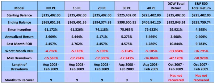
Figure 10a shows the performance of the base case period (December 31, 1999 to December 31, 2010) with the assumed dividend rate of the model changed to 1%.

Best Month ROR 4.457% 4.762% 4.457% 4.575% 4.286% 10.844% 9.783%

Worst Month ROR -4.797% -5.118% -5.103% -5.164% -5.105% -13.884% -16.795%

Max Drawdown -15.565% -17.284% -17.300% -17.241% -16.868% -47.120% -50.920% Length of Drawdown Aug 2008 - Feb 2009 Aug 2008 - Feb 2009 Aug 2008 - Feb 2009 Aug 2008 - Feb 2009 Aug 2008 - Feb 2009 Oct 2007 - Feb 2009 Oct 2007 - Feb 2009 Months to Recover 9 9 9 9 9 Has not recovered Has not recovered

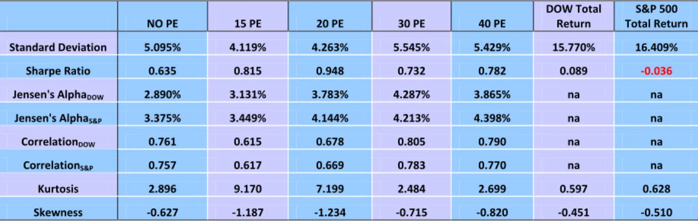
Figure 10b shows the statistical results of the base case period December 31, 1999 to December

31, 2010 with the assumed dividend rate of the model changed to 1%.

Kurtosis 2.860 9.123 7.130 2.449 2.667 0.597 0.628

(47)

Figure 11a shows the performance of thebase case period December 31, 1999 to December 31, 2010 with the assumed dividend rate of the model changed to 0%.

Best Month ROR 4.517% 4.764% 4.474% 4.575% 4.350% 10.844% 9.783%

Worst Month ROR -4.842% -5.162% -5.170% -5.285% -5.170% -13.884% -16.795%

Figure 11b shows the statistical results of thebase case period December 31, 1999 to December

31, 2010 with the assumed dividend rate of the model changed to 0%.

Kurtosis 2.896 9.170 7.199 2.484 2.699 0.597 0.628

Skewness -0.627 -1.187 -1.234 -0.715 -0.820 -0.451 -0.510

Figures 12, 13, and 14 show the performance and statistical results of the model from Dec1999 to Dec 2010 with the minimum premium option variable changed from 1.5% to 2.5% to 5%.

(48)

Figure 12a shows the performance of the base case period December 31, 1999 to December 31, 2010 with the minimum option premium set to 1.5%.

Model NO PE 15 PE 20 PE 30 PE 40 PE DOW S&P 500

Starting Balance $225,402.00 $225,402.00 $225,402.00 $225,402.00 $225,402.00 $225,402.00 $225,402.00

Ending Balance $395,117.73 $346,862.76 $366,379.04 $384,568.60 $382,460.32 $292,843.61 $235,759.74

Since Inception 74.446% 53.141% 61.757% 69.788% 68.857% 29.921% 4.595%

Annualized Return 5.189% 3.950% 4.469% 4.930% 4.878% 2.408% 0.409%

Best Month ROR 3.872% 4.054% 4.235% 3.991% 4.021% 10.844% 9.783%

Worst Month ROR -3.504% -3.374% -3.782% -3.614% -3.642% -13.884% -16.795%

Max Drawdown -10.203% -8.403% -10.931% -10.507% 10.870% -47.120% -50.920% Length of Drawdown Aug 2008 - Feb 2009 Sep 2008 - Feb 2009 Aug 2008 - Feb 2009 Aug 2008 - Feb 2009 Aug 2008 - Feb 2009 Oct 2007 - Feb 2009 Oct 2007 - Feb 2009 Months to Recover 6 5 6 6 6 Has not recovered Has not recovered

Figure 12b shows the statistical results of the base caseperiod December 31, 1999 toDecember

31, 2010 with the minimum option premium set to 1.5%.

Model NO PE 15 PE 20 PE 30 PE 40 PE DOW S&P 500

Standard Deviation 3.044% 2.370% 2.729% 2.988% 3.187% 15.770% 16.409%

Sharpe Ratio 1.376 1.245 1.271 1.315 1.217 0.089 -0.036

Kurtosis 6.649 16.195 13.269 7.958 6.030 0.597 0.628

(49)

Figure 13a shows the performance of the base case period December 31, 1999 to December 31, 2010 with the minimum option premium set to 2.5%.

Best Month ROR 4.198% 4.346% 4.297% 4.204% 4.180% 10.844% 9.783%

Worst Month ROR -4.446% -4.497% -4.741% -4.549% -4.523% -13.884% -16.795%

Max Drawdown -15.153% -14.634% -15.580% -15.899% -15.819% -47.120% -50.920% Length of Drawdown Aug 2008 - Feb 2009 Sep 2008 - Feb 2009 Aug 2008 - Feb 2009 Aug 2008 - Feb 2009 Aug 2008 - Feb 2009 Oct 2007 - Feb 2009 Oct 2007 - Feb 2009 Months to Recover 9 7 9 9 9 Has not recovered Has not recovered

31, 2010 with the minimum option premium set to 2.5%.

Kurtosis 3.438 10.974 9.094 4.010 4.056 0.597 0.628

(50)

Figure 14a shows the performance of the base case period December 31, 1999 to December 31, 2010 with the minimum option premium set to 5%.

Best Month ROR 4.978% 4.946% 4.839% 4.695% 4.887% 10.844% 9.783%

Worst Month ROR -5.596% -6.047% -5.295% -5.272% -5.822% -13.884% -16.795%

31, 2010 with the minimum option premium set to 5%.

Kurtosis 1.549 8.323 4.136 2.188 2.001 0.597 0.628